This section explains how the predicted heat losses and gains in the system were calculated. It is an overview of the heat loss estimation performed on the components of this system. The sub sections for each component show the equations selected, tells why they were used, and explains the assumptions made. The results are then entered into a large energy balance to determine the system heating and storage needs. An analysis was performed on the optimum placement of a solar panel to determine the approximate in-flux of power. A detailed walkthrough of the calculations performed and numerical results for each component are available as MathCAD 2000 files, and can be downloaded from links after each section.
All heat loss calculations were performed following the same base format.
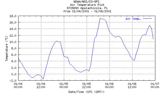
A calculation for a single condition was done for each part of the system to
estimate the rate of heat loss in watts during the coldest part of the coldest
day in 2001 as recorded by NOAA. This information was collected in Apalachicola,
about 60 miles from the test site. The coldest conditions were selected for the
calculations to attempt to predict the heat losses during a worst-case scenario
in the weather. The air temperature information used in these calculations is
shown in the figure 5.1 below. The data for January 4 is being employed.
Figure
5.1: Temperatures 2001
The
ambient conditions were set at 10°F using the weather data (a typical day
during the winter months in Florida is generally 15°F to 25°F warmer at its
coldest point even during arctic fronts). A thermal resistance network was
defined for each component based on the material and manner in which it will be
insulated during system construction. This thermal resistance network included
estimations of heat transfer coefficients for the contact areas between flowing
water and pipes or tanks, and depend on flow rates through the various
components.
After
the ambient conditions and the thermal resistance networks were completed for
each component, the rate of heat loss was determined. This value, given in watts
at the end of each MathCAD worksheet, is how quickly energy in the component is
being lost to the atmosphere in the conditions of the coldest part of the
coldest day of 2001.
Once
the rate of heat loss of each component was determined, the values were added up
to find the rate of energy loss of the total system. Since the target
aquaculture tank temperature is 77°F, if the ambient conditions are at or above
this value, heat loss will be zero. Using these two points as a foundation, a
linearized representation of the rate of heat loss from the system was graphed
against a range of ambient conditions in figure 5.2.
Figure 5.2: System Energy Loss
It
is reasonable to estimate the system heat losses in a linear manner because the
actual heat losses will be lower as the ambient temperature approaches the
temperature of the water in the aquaculture tank. Heat transfer is heavily
dependent on a temperature difference. The slight overestimation of heat losses
this method produces acts as a margin of safety in the design of the system.
The next step was to attempt to predict the total energy loss over the
course of a day. The approach to this is similar to using the trapezoid rule to
perform a numerical estimation of an integral.
The
NOAA data in figure 5.1 was once again consulted. The temperature data from
January 1, 2001 was used to find the ambient air conditions at eight points
throughout the day, representing three-hour blocks of time. The indicated
temperature from the NOAA website and the linearized interpolation of rate of
heat loss vs. temperature was used to estimate an average rate of heat loss for
that three hour block, and a total energy loss for the block was calculated.
The
eight energy loss totals from these blocks were then totaled to show a predicted
total energy loss under the most adverse conditions during the coldest expected
conditions. These blocks are represented in figure 5.3 below.
Figure
5.3: Energy Lost During the Coldest Day (3hr. blocks)
Adding
up the values of these blocks is similar to adding up the areas in a number of
trapezoids when employing the trapezoid rule. It approximates a much more
complex integration of the energy lost over a twenty-four hour period.
This
yields a predicted total energy loss of 12900kJ over the course of a day similar
to the coldest day on record in 2001. To be able to keep the water temperature
at 77°F in the aquaculture tank, the solar collection and an energy storage
system must be able to acquire and store 12900kJ (3.58kW*hr) over the course of
the day under the least favorable conditions.
The
Cp value for water is 4.18kJ/kg*K, and the storage system capacity is
approximately 1800 liters (about 1800kg @ 25°C). To have sufficient heat
transfer between the heat storage tank and the aquaculture tank, the temperature
difference between the two should be at least 3°C. The heat storage tank holds
around 7500kJ of useable energy for each degree Centigrade that the solar
collector raises the water temperature above 28°C.
To
provide a margin of error for the system, the heat storage tank target
temperature is a minimum of 30°C (86°F) to be able to maintain the aquaculture
system at 25°C (77°F) for one twenty-four hour period. To be able to sustain
the system for two days without further solar collection the heat storage tank
will need to be raised to at least 33°C (91.5°F).
If
the system goes for more than forty-eight hours with no solar heat collection in
the event of a long storm or very overcast days, supplemental heating will need
to be employed. This approach sets all conditions and assumptions based on a
worst-case scenario. There are typically only a couple of days per year that the
described weather conditions are encountered.
For
the aquaculture tank, the losses through the bottom of the tank were negligible
as it is well insulated and the ground will be close to the target temperature
in comparison with the outside air temperature. The top of the tank was treated
as if it were additional wall. This was done because the tops of the tanks are
insulated in a manner similar to the sides. There is a 6” gap between the
insulation and the water surface.
The
thermal network for the sidewalls of this tank is identical to the thermal
resistance network for the heart storage tank. Both have water flowing across a
¼” thick plastic wall that is covered by a 2” thick Styrofoam sheet with a
reflective metallic backing. The joints are sealed with duct tape. Perfect
contact between the Styrofoam and the plastic wall are assumed.
The
conduction on the inside of the tank was addressed first. In this worksheet, the
high flow rates required for the filtration system the aquaculture requires
caused the flow inside the tank to model as turbulent. Using the value of the
Reynolds number and water properties at 25°C, the Nusselt number and a
corresponding heat transfer coefficient were found.
The
convection on the outside of the tank between the outer wall and the atmosphere
was addressed next. This was accomplished using the biot number to estimate the
Rayleigh number, which was in turn used to find the Prandl and then the Nusselt
number. These non-dimensional parameters were then used to estimate a heat
transfer coefficient value for the outside of the tank.
Using
the calculated heat transfer coefficients and the known thermal properties of
the plastic wall and Styrofoam, an overall thermal resistance value was found
and a heat loss rate per square meter of wall was determined by using the
temperature values for the water and the air. This value was multiplied by the
actual wall and lid area to find the expected heat loss rate for the aquaculture
tank.
The
heat loss through the solar panel from convection was ignored. This was done for
two reasons. First, the solar panel will be insulated on the back and covered on
the top with a material that has high emmissivity and low thermal conduction,
such as plexiglass. Secondly, for the purpose of solar panel evaluation, the
actual collected energy will be determined empirically.
Heat
gained through the solar collector will be determined experimentally.
Performance data on solar collectors is generated in a controlled environment
and is useful only for comparison between two different solar collectors. The
number of parameters that would be nothing more than a guess in calculating a
heat collection value would make any result worthless.
Instead,
the amount of energy needed has been determined, and the existing solar
collector will be tested to determine if it can meet the system requirements. If
it cannot, another collector design will be tested, an additional collector will
be mounted, or a supplemental heating source such as resistive heating or gas
heating will be employed.
The
heat lost through the pipes is dependent on the thermal resistance network, the
flow rate through the pipes, and the temperature of the water in the pipes. All
plumbing in the system will be done with sch40 PVC pipe, and will be insulated
with the same preformed foam product. Therefore the insulation will be the same,
but flow and temperature values will differ.
The
temperature of the water in these pipes (77°F) is less than that of the water
in the heat storage system, but the flow rates are higher. The losses in these
pipes were calculated in a manner similar to the tank sidewall heat losses.
Aquaculture
Tank Pipe Heat Loss
The temperature of the water in the heat storage system was set at 100°F to find maximum heat loss. The actual temperature should be less than this in the system, but the higher temperature is in line with the trend of overestimating losses and performing calculations in a worst-case scenario.
Energy
Storage Pipe Heat Losses
The
approach to determining the losses through the heat storage system tank was very
similar to the procedure described previously for the aquaculture tank. The same
assumptions about material properties, geometry, and perfect contact were kept.
The
flow rates through the system are lower, and the flow models as laminar rather
than turbulent. This changes the method for predicting the inside wall heat
transfer coefficient. Details are available in the Appendix C.
An
estimated 79.2 kJ will be irradiated from the sun to the solar panel during
daylight hours. This estimate is
made with the assumption that the solar panel is at an optimum position and the
day in question for gathering energy is clear.
The energy irradiated to the solar panel is determined using a table of
constants in appendix D and empirical equations found in the 1997 ASHRAE
handbook. Specifics on the
calculations are also explained in appendix D.