Experiment
6
Velocity
Field Measurements of a Rectangular Jet
Download
Experiment Description
Objectives
There
are two main objectives of this experiment. The first goal is to perform
a calibration to obtain the relationship between the voltage output from
a hot-wire/film and the fluid velocity to which the hot wire is exposed.
The second objective is to study the fluid dynamic properties of a rectangular
air jet. The first objective is achieved by performing a static calibration
where the hot wire is exposed to a fluid stream with a known velocity and
the output voltage of the hot wire/film signal conditioning circuit is
recorded. In the second part of this experiment, insight into important
physical properties of rectangular jets, such as jet growth or spreading,
will be gained by measuring the velocity profiles in the jet at various
locations, thus examining its development in space.
Theoretical
Background
Hot-Wire/Film
Anemometer
Hot-Wire
and Hot-Film anemometers are commonly used to measure fluid velocities.
They have excellent dynamic response and are therefore frequently used
to measure mean as well as unsteady components of velocity. Hot wires and
hot films are both very delicate instruments which can be easily damaged.
Therefore, they are generally used for measurements in clean (i.e. no fluid
borne particles such as dust), low-speed flows. However, if designed properly
and handled carefully along with a little luck- they can be used in high-speed,
even supersonic, flows. The principle of operation for both hot wire and
hot film anemometers are the same, hence even though the following discussion
refers to hot wires, it is equally applicable to hot films.
Hot
wires can be operated in two basic modes, the constant current mode
and the constant temperature mode. Both modes employ the same physical
principle of forced convection heat transfer where the very thin wire is
modeled as an infinitely long cylinder.
Constant
Current Mode:
In
the constant current mode, a nearly fixed electric current flows through
the wire, which is exposed to the flow velocity. The wire attains an equilibrium
temperature resulting from the balance between internal heat generation
due to electrical resistance (Joule heating) and the convective heat loss
from the wire to the moving fluid. The wire temperature must adjust itself
to changes in the convective losses until a new equilibrium temperature
is obtained. Since the convection coefficient is a function of the flow
velocity, the equilibrium wire temperature is a measure of the velocity.
The wire temperature can be measured in terms of its electrical resistance
where the relationship between the resistance and temperature is known
a priori.
Constant
Temperature Mode:
In
the constant-temperature mode, the mode used in this experiment, the current
through the wire is adjusted to maintain a constant film temperature. The
constant temperature is maintained by using a feedback circuit, details
of which are beyond the scope of this lab. Based on the energy balance
discussed in the next section, it should be clear that the current required
to maintain the wire at a constant temperature, is proportional to the
convective heat loss and can therefore be used to measure the flow velocity.
Energy
Balance for a Hot Wire:
Under
equilibrium conditions, the energy balance equation of a hot-wire is given
as:
 (1)
(1)
where
I is the current, Rf is the wire resistance, Tf is
the wire temperature, Ta is the surrounding fluid (in this case,
air) temperature, h is the convection coefficient and A is the surface
heat transfer area. For a wide range of velocities, the convection heat
transfer coefficient, h, can be related to the instantaneous convection
velocity V. Based on empirical evidence, a correlation between the current,
wire resistance and the fluid velocity, known as King's Law, has
been established. Kings law has been validated for hot wires (and hot
films) operating in constant temperature mode over a wide range of velocities.
In one form, King's law can be expressed as:
 (2)
(2)
where
A0 and A1 are considered to be constants under fixed
operating conditions. For a properly designed system, the supplied current
can be directly related to the anemometer output voltage, E, allowing us
to write Kings Law in a slightly different form as follows:
 (3)
(3)
where
C0 and C1 are constants and E0 is the
voltage measured at zero jet velocity. In the first part of the experiment
you will determine value of the constants C0 and C1.
Note that although V1/2 is most commonly used, a more general
form of equations 2 or 3 would instead include the velocity dependence
as Vn, where the exponent n can range between 0.45 and
0.55 depending on the wire and the flow conditions over which the wire
is to be used.
Flow
Properties of a Rectangular Jet
A
jet is formed by flow issuing from a nozzle into ambient fluid, which is
at a different velocity. If the ambient fluid is at rest the jet is referred
to as a free jet; if the surrounding fluid is moving, the jet is called
a coflowing jet. A jet is one of the basic flow configurations which has
many practical applications such as in jet engines, combustors, chemical
lasers, ink-jet printer heads, among others. Figure 1 illustrates some
essential features of a jet. The velocity at the exit of the nozzle of
a typical laboratory jet has a smooth profile and a low turbulence level,
about 0.1% - 0.5% of the mean velocity. Due to the velocity difference
between the jet and the ambient fluid, a thin shear layer is created.
This shear layer is highly unstable and is subjected to flow instabilities
that eventually lead to the formation of large-scale vortical structures
(see
Figure 1). The interaction of these structures produces strong flow fluctuations,
entrains ambient fluid into the jet flow and enhances the mixing. The shear
layer and consequently, the jet spread along the direction perpendicular
to the main jet flow.
The
central portion of the jet, a region with almost uniform mean velocity,
is called the potential core. Because of the spreading of the shear
layer, the potential core eventually disappears at a distance of about
four to six diameters downstream from the nozzle. The entrainment process
continues further beyond the end of the potential core region such that
the velocity distribution of the jet eventually relaxes to an asymptotic
bell-shaped velocity profile as illustrated in Figure 1. Also shown in
Figure 1 is the half-width of the jet, y1/2, defined as the
distance between the axis and the location where the local velocity
equals half of the local maximum or centerline velocity, U0.
The increase in the jet half-width with downstream distance provides a
measure of the spreading rate of the jet. Due to the spreading, the jet
centerline velocity, Vc, decreases downstream beyond the potential core
region.
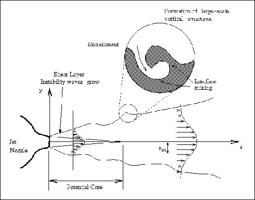
Figure
1.Schematics of a free jet flow
and its downstream development
IMPORTANT
NOTE: The hot-wire probe is extremely fragile!
Simply simply touching the tip of the probe can break it. Therefore, it
must be handled very carefully. The lab instructor will set up the probe
and also show you how to use it. Do not handle the probe on your
own, without the instructors permission.
Apparatus
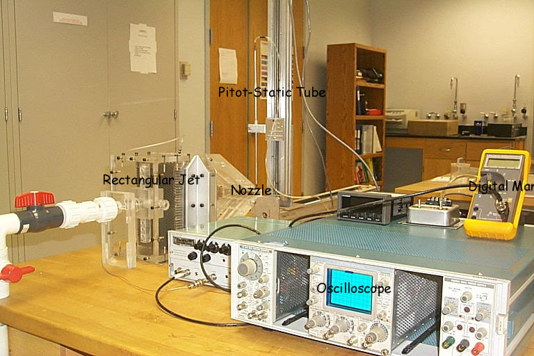
The
following apparatus will be used for this experiment:
1.
A rectangular jet, with a nozzle of dimensions 6 cm X 1 cm.
2.
An air pump to force air stream through the jet nozzle.
3.
A hot-wire anemometer, and its associated digital circuitry.
4.
A pitot-static tube and a digital manometer.
5.
A Pentium-based PC with LabVIEW software and an associated ADC card.
6.
An oscilloscope.
Experimental
Procedure
Calibration
of the Hot Wire
1. Turn
on the air pump to establish the jet flow. Estimate the jet exit velocity
by measuring the stagnation pressure inside the reservoir chamber. The
difference between the stagnation pressure and the free stream static pressure
is a good approximation of the dynamic pressure of the exit stream.
2. Carefully
move the hot-wire/film probe into the potential core region of the jet
where the velocity is relatively uniform and fluctuation free. Confirm
this by monitoring the output signal from the hot-wire on the oscilloscope.
3. Connect
the anemometer output to the analog-to-digital converter (ADC) and the
oscilloscope. Determine the time-averaged anemometer voltage output using
the ADC and the LabVIEW software.
4. Record
the ADC output.
5. Repeat the
calibration procedure for the velocity range from 0 (the lowest velocity
available to the maximum velocity.
6. Record
10 data points over this velocity range.
Jet Centerline
and Cross-Stream Velocity Profile Measurements
1.
Set the dynamic pressure of the jet exit velocity at the maximum stable
setting (usually between 0.06 and 0.07 psi). Note: The digital pressure
gage has an upper limit of 0.1 psi. Do not overload the unit!
2.
Beginning at a position approximately at the jet nozzle, move the pitot-static
probe along the center axis of the jet. Measure the jet centerline velocity
at 1cm intervals for 31 data points.
3.
Move the probe to a downstream location of x/D = 4. (The height D of the
jet nozzle is 1cm) Measure the cross-stream velocity profile by using the
computer-controlled traverse to move the probe in the vertical direction
and recording the output using LabVIEW.
4.
A total of 8 points with a 1 mm increment should be measured.
5.
Move the prove to another downstream location at x/D = 10 and measure the
velocity profile.
6.
Record
the ADC output for this location also.
7.
Use 8 points and a 3 mm increment.
Questions
to be answered
1.
Use the data collected in the calibration portion of the experiment, verify
Kings Law. Plot (E-E0)2 vs.  and determine the constants C0 and C1. Discuss the
types of errors present in the experiment.
and determine the constants C0 and C1. Discuss the
types of errors present in the experiment.
2.
Plot the variation of the jet velocity along the center axis, that is,
Vc/Vexit vs. x/D. Discuss your results.
3.
Can you identify the end of the potential core based upon your time-averaged
velocity data?
4.
Plot the time averaged mean velocity profiles at x/D=4, 10, 20, and 30,
that is V(y)/Vc vs y/D. Plot the variation of the half jet width, y 1/2
vs x/D. Discuss the results of both plots.