EML 5060 Analysis in Mechanical Engineering 12/10/13
Closed book Van Dommelen 10-12 noon

Solutions should be fully derived showing all intermediate results, using class procedures. Show all reasoning. Bare answers are absolutely not acceptable, because I will assume they come from your calculator (or the math handbook, sometimes,) instead of from you. You must state what result answers what part of the question if there is any ambiguity. Answer exactly what is asked; you do not get any credit for making up your own questions and answering those. Use the stated procedures. Give exact, fully simplified, answers where possible.

One book of mathematical tables, such as Schaum's Mathematical Handbook, may be used, as well as a calculator, and a handwritten letter-size formula sheet.

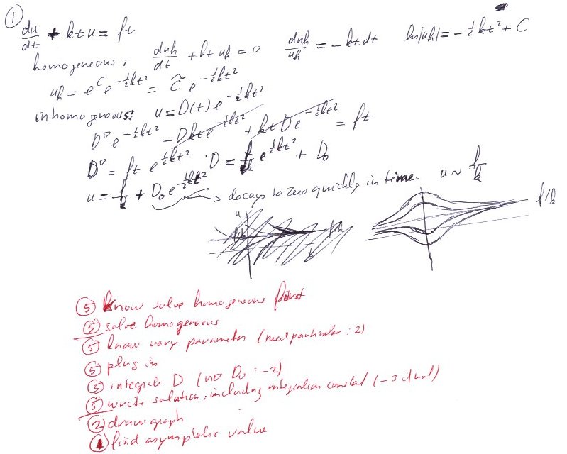
1. Background: Consider a sphere moving in a viscous fluid. The viscosity of the fluid is increasing linearly in time as its gets hotter. A force is applied that grows proportional to the viscosity. The velocity $u$ of such a sphere is described by
   
   $$\frac{{\rm d}u}{{\rm d}t} + k t u = f t$$
   
   
   where $k$ and $f$ are positive constants.

   Question: Solve the above system using the class procedure for linear 1st order equations. Graph some representative solution curves versus time. What can you say about the long-time behavior of the velocity?

   Solution.

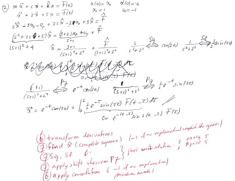
2. Background: The Laplace transform is one way of solving complicated dynamical systems. One strength is its capability of analyzing the stability properties. The simplest dynamical system is of course the one-dimensional spring mass system
   
   $$m \ddot x + c \dot x + k x = F \qquad x(0) = x_0 \quad \dot x(0) = v_0$$
   
   
   where $m$ is the mass, $c$ the damping constant, $k$ the spring constant, and $F$ the applied force.

   Question: Solve the above system using the Laplace transform if $m=1$, $c=2$, $k=5$, and $F$ is some given function of time. Take $x_0=1$ and $v_0=-1$.

   A table of Laplace transforms is attached. Everything not in this table must be fully derived showing all reasoning. The convolution theorem may only be used where it is absolutely unavoidable. Do not use any complex numbers in your analysis (besides $s$.)

   Solution.

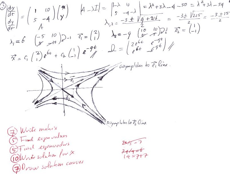
3. Background: In steady fluid flows, the fluid motion satisfies, of course, ${\rm d}{\vec r}/{\rm d}t=\vec v$. Near a stagnation point, the right hand side can be linearized to show the local motion.

   Question: Solve using class procedures for 1st order systems:
   

   $$\frac{{\rm d}x}{{\rm d}t} = x + 10 y \qquad \frac{{\rm d}y}{{\rm d}t} = 5x -4 y$$
   
   
   which would be a possible example in two dimensions.

   Draw the solution curves in the $x,y$-plane very neatly and quantitatively reasonably accurately. You should have 2 examples of each different type of curve, or 1 if there is just one curve of that type. Be sure to put an arrow in the direction of motion on each curve.

   Make sure that you check your algebra carefully. You do not get credit for making the wrong graph.

   Solution.

Table 1: Properties of the Laplace Transform. ($k,\tau,\omega>0$, $n=1,2,\ldots$)