EML 3002L M.E. Tools Lab 11/21/17
Matlab Exam 2 Van Dommelen 12:30-1:45 pm

NO CELL PHONES, HEADPHONES/BUDS, NO CALCULATORS. SAVE FREQUENTLY. SAVE BEFORE PUBLISHING!!!

ONLY MATLAB MAY BE ACTIVE ON YOUR COMPUTER.

After translation into mathematics, only Matlab may be used to solve the full problem as posed. Use the appropriate procedures as covered in the lectures. Use appropriate variable names that can be clearly understood by the grader. Use appropriate comments. Acrobat may only be open at the end, when you are ready except for publishing and actively looking at main.pdf with it.

“Open notes: print-outs of lectures and homeworks allowed. You can also use your own homework .m files.”

1. The following system of $n$ equations in $n$ unknowns $T_1,T_2,\ldots,T_n$ could arise in the computation of unsteady heat conduction in a ring.
   

   $$T_n - 3 T_1 + T_2 = 1$$ (1)

   $$T_1 - 3 T_2 + T_3 = 2$$ (2)

   $$T_2 - 3 T_3 + T_4 = 3$$ (3)

   $$T_3 - 3 T_4 + T_5 = 4$$ (4)

   $$\vdots$$ (5)

   $$T_{n-2} - 3 T_{n-1} + T_n = n-1$$ (6)

   $$T_{n-1} - 3 T_n + T_1 = n$$ (7)

   
   
   Take $n=5$ for now, then
   

   $$T_5 - 3 T_1 + T_2 = 1$$ (8)

   $$T_1 - 3 T_2 + T_3 = 2$$ (9)

   $$T_2 - 3 T_3 + T_4 = 3$$ (10)

   $$T_3 - 3 T_4 + T_5 = 4$$ (11)

   $$T_4 - 3 T_5 + T_1 = 5$$ (12)

   
   
   However, your code should still work correctly if you change $n$ (variable n) into a bigger value, without other changes. Initialize the matrix of this system of equations to zeros, then use a for loop over the equations to put in the nonzero elements. Be careful with the first and last equations as they have a variable out of order. Also create the right hand side vector. Print out matrix and right hand sides as [A,b].

   Use an if statement to check whether the system of equations has a reasonably accurate solution. If it does, your code should solve the system and print out the solution. If it does not, your code should print an appropriate warning. This should again continue to work for whatever value is given to variable n.

   Grading

2. Using the Symbolic Math Toolbox, do the following:
   1. Use ezplot to plot the function $xe^{-x^2}$ from $-2$ to 2. Turn on the grid.
   2. Find the partial fraction expansion of the ratio
      
      $$s/(s^3+4s^2+s+4)$$
      
      

   3. For the quartic
      
      $$Q = x^4 - 2 x^3 + 22 x - 9$$
      
      
      1. Let Matlab find the exact roots, i.e. the exact four values of $x$ where $Q$ is zero.
      2. Let Matlab factor the quartic $Q$. Your result should take the form of parenthetical expressions multiplied together.
      3. Let Matlab find the derivative and antiderivative of the quartic $Q$.
      4. Let Matlab find the exact integral of the quartic $Q$ between the limits 0 and 2.

   Grading

3. The maximum lift produced by a small plane (flaps up) increases with velocity as shown by the below measurements:

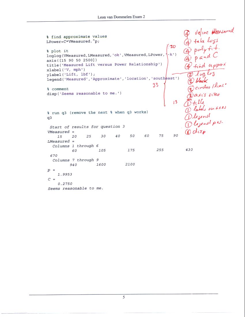
   $V$ mph:	15	20	25	30	40	50	60	75	90
   $L$ lbf:	60	105	175	255	430	670	940	1600	2100

   Try to approximate these measurements by a power relationship $L=CV^p$ where $C$ and $p$ are constants. Plot both the measured data, as black circles, and the approximation, as a solid black line, in a log-log graph. Horizontal axis from 15 to 90, vertical axis from 50 to 2500. Title “Measured Lift versus Velocity Relationship”. Appropriate labels along the axes. Legend Measured” and “Approximate, placed in the southeast corner. Use disp to comment on how well you think the fit is.

   Grading

Solutions without credit distribution.
Solutions with credit distribution.