for the time
The equation above determines the time ![]() it takes for a car wheel
that rolls off a step down of size
it takes for a car wheel
that rolls off a step down of size ![]() to hit the ground behind the
step. In particular the left hand side is the distance traveled
downwards by the wheel before it hits the ground after the step, and
the right hand side is the total size of the step down.
to hit the ground behind the
step. In particular the left hand side is the distance traveled
downwards by the wheel before it hits the ground after the step, and
the right hand side is the total size of the step down.
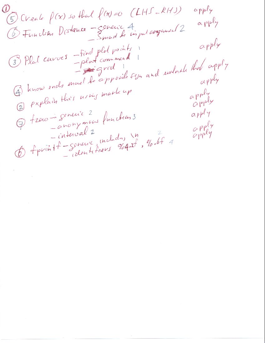
Define a function that can be used by fzero to find the
time ![]() at which the equation above is satisfied for given
at which the equation above is satisfied for given ![]() .
The function should work unchanged for any value of
.
The function should work unchanged for any value of ![]() , so do not
set a value for
, so do not
set a value for ![]() inside the function. Call the function
Distance, as surely you recognize that it is really the
vertical distance
inside the function. Call the function
Distance, as surely you recognize that it is really the
vertical distance ![]() between the wheel and the ground behind the
step.
between the wheel and the ground behind the
step.
Make sure your function allows input argument ![]() to be an array
instead of a scalar.
to be an array
instead of a scalar.
Now plot this function using 51 ![]() values from 0 to 5, for the two
values of
values from 0 to 5, for the two
values of ![]() equal to 0.25 and 0.75. Use a grid.
equal to 0.25 and 0.75. Use a grid.
Use mark-up comments to explain why the interval from 0 to 5 will
work for sure in both cases to find the time ![]() that the wheel
reaches the ground.
that the wheel
reaches the ground.
Then find the two times using fzero using that interval and print them out as
For S = 1.12, t = *.123456 (interval [1 1]).where the star means whatever digits MATLAB want to print out, and 12... is a count of digits to output. Absolutely no data numbers inside the FORMATSTRING, just format descriptors.
Make sure that you change FUNNAME or Blah into Distance in the header of q1.m before publishing! Careful: do not mess up the format of the two lines involved while doing this!
That means that if we integrate the ratio
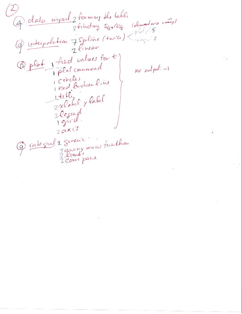
Below is an extract of the saturated data of water given in
the Sonntag book:
Copy this table as is into your solution in q2.m and then find the integrand
Spline interpolate this integrand at 101 plot temperatures from 5 to
25. Then plot the 5 values of the integrand against the 5
temperatures as little black circles, and the spline interpolate as
a red broken (dashed) line. Use title “Clausius-Clapeyron
Integrand”, axis labels T
and
sfg/vfg
, use a grid, and a legend
tabulated,” “spline interpolate
placed
in the bottom right of the plot. Let MATLAB choose the horizontal
axis limits, but force it to use a vertical axis from 0 to 0.2.
Finally, integrate the spline interpolate from temperature 5 to 25
and compare the pressure difference between 5 and 25 that you get
this way with the exact
pressure difference that you
get from the above table.
Also integrate the linear interpolate and compare that with exact.
Each time the reaction occurs, it removes two
| (1) |
where
where
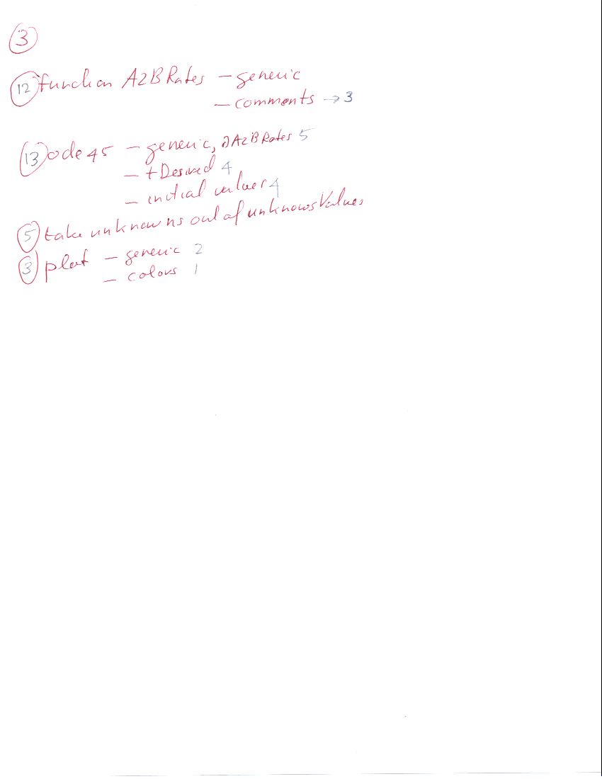
Solve the above system of three ODE using ode45 for 101
times ![]() from 0 to 100. Use variable names cA,
cB, and cA2B for
from 0 to 100. Use variable names cA,
cB, and cA2B for ![]() ,
, ![]() , and
, and ![]() respectively. Take the initial conditions to be that
respectively. Take the initial conditions to be that ![]() ,
,
![]() , and
, and ![]() .
.
Call the function needed by ode45
A2BRates
. Show in your first command in
q3.m that help A2BRates explains what the function
does and what its input and output arguments are.
Plot the concentrations against time, using red for ![]() , blue for
, blue for
![]() , and black for
, and black for ![]() .
.
Make sure that you change FUNNAME into A2BRates in the header of q3.m before publishing! Careful: do not mess up the format of the two lines involved while doing this!