| Fall 2007 Homework Problems | © Leon van Dommelen |
|
|
| Fall 2007 Homework Problems | © Leon van Dommelen |
|
|
plot and maybe hold
commands. Verify that the highest Reynold number has the lowest
wall shear.
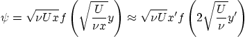
Function ![]() can in principle be found by integrating function
can in principle be found by integrating function
![]() of the previous homework, but you saw what a mess that
was. It is neater to simply integrate the system of ordinary
differential equations satisfied by
of the previous homework, but you saw what a mess that
was. It is neater to simply integrate the system of ordinary
differential equations satisfied by ![]() and
and ![]() :
:
Run the program and verify that recirculatory streamlines occur at the rear of the cylinder, as a first step in creating the wake.
Now copy the program to another name and remove the second order term of Blasius. Remove all traces, such as variables that are no longer used and update all comments. Replot, and comment on why the term added by Blasius is important for understanding the flow development.
Now copy the program to another name and remove the first order,
Stokes second problem, term too. Comment on the effect that this
term has compared to the potential flow streamlines. (You can let
this program inherit the ![]() -values from the previous one, but add a
comment near the start of the file that it needs to do so.)
-values from the previous one, but add a
comment near the start of the file that it needs to do so.)
zeta_vals returned by
ode45. Since the vorticity values at high Reynolds numbers
are large, you may want to plot from -110 to 110 in increments of
20. In particular, avoid plotting the zero vorticity line since it
is extremely round-off sensitive. Comment on where the vorticity
can and cannot be found in high-Reynolds number flow. According to
the Stokes second problem approximation, the boundary layer
thickness would be the same along the cylinder, take it
blaspsi.m found here plots
the streamlines around a semi-infinite flat plate. Using the matlab
hold and plot commands, add the displacement
thickness curve x. Are the streamlines
parallel to the plate with the displacement thickness added? If
not, why not? To better see which streamlines are parallel to the
thickened plate, also plot displacement curves shifted upwards by
0.025, 0.05, and 0.1, in green. Comment on in what sense the effect
of the boundary layer is to thicken the plate by the displacement
thickness.
You may wonder about the use of ``optimal coordinates.'' The
Blasius solution is written in terms of conformally mapped
coordinates