Equations

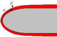
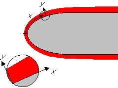
Boundary layer coordinates:

Note that despite their names, x and y are not Cartesian coordinates.

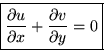
Laminar boundary layer equations:

Seen on the small transverse boundary layer length scale, the boundary layer coordinate system looks approximately Cartesian:

As a result, to first approximation, there are no terms related to the curvature of the coordinate system introduced in the governing equations. In addition, some terms can be neglected since the boundary layer is thin and is small. What is left (in 2D) is:

Continuity:

which is unchanged compared to the 2D incompressible equations in Cartesian coordinates.

x-Momentum:

since the viscous term is negligible for small . Note that the viscous term is not negligible since the smallness of is balanced by the fact that u varies rapidly in the direction across the boundary layer, wich has a typical thickness .

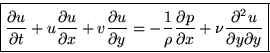
y-Momentum:

Almost all terms can be ignored since the transverse velocity v is small. It follows that the variation of the pressure across the thin boundary layer is negligible; p=p(x,t).

An example of a boundary layer solution is Stokes' second problem, the impulsively started flat plate, in which v=0 and . This is an exact solution of the Navier-Stokes, as well as of the boundary layer equations. Note that the thickness of this boundary layer is indeed proportional to .

Boundary conditions at a solid, stationary, impermeable wall:

Boundary conditions above the boundary layer follow from the fact that directly above the boundary layer, there is a ``matching'' region in which both the boundary layer solution and the potential flow solution are valid approximations:

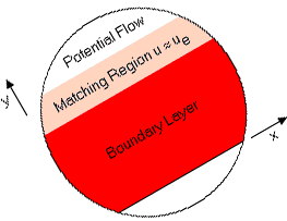
In the matching region, as far as the potential flow is concerned y is small, but as far as the boundary layer solution is concerned, . Since y is small, the velocity u=u_e(x,t) is approximately the wall slip velocity found from the potential flow solution (in which the thin boundary layer is ignored.) But the velocity u_e must also be the velocity in the boundary layer solution for .The same holds for the pressure:

Note that is constant, since the Bernoulli law applies in the matching region.

04/07/00 0:30:06 04/10/00 0:01:10 04/12/00 0:00:32