|
|
|
To: 8.2.5 Drag force |
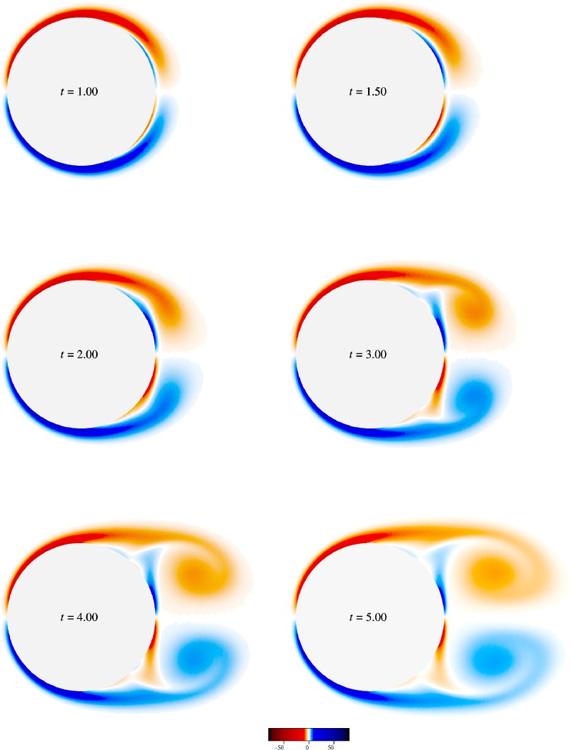
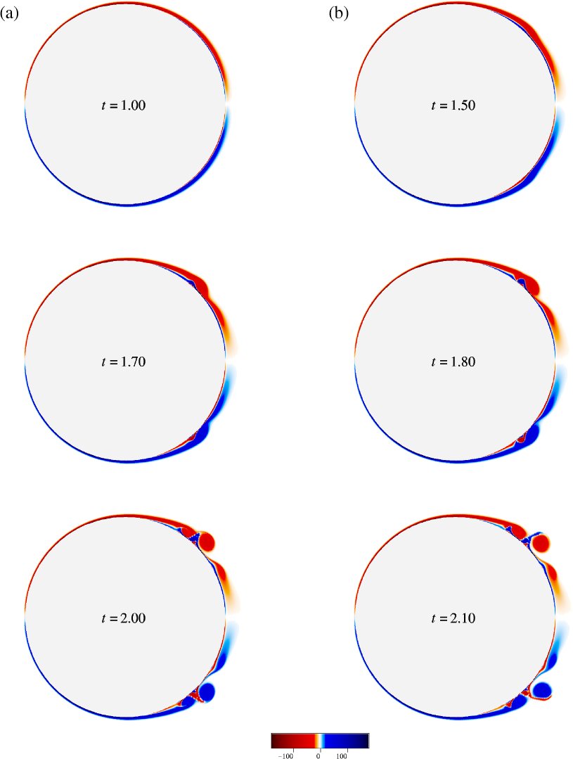
When the circular cylinder is impulsively set into motion, the initial flow around it is irrotational [14]. All circulation occurs in a vortex sheet on the cylinder surface at that instant [130]; this vortex sheet diffuses out into the flow for later times.
The evolution of the vorticity field is shown in figures
8.16, 8.17, 8.18 and
8.19 for ![]() , 3,000, 9,500, and 20,000 respectively.
For all these Reynolds numbers, by time
, 3,000, 9,500, and 20,000 respectively.
For all these Reynolds numbers, by time ![]() when the cylinder has
moved a distance of one radius, the flow
at the rear surface of the cylinder is in the upstream direction.
This upstream flow (or flow
reversal) is indicated by a vorticity sublayer of opposite sign
(color in the figures)
to that of
the main boundary layer above it.
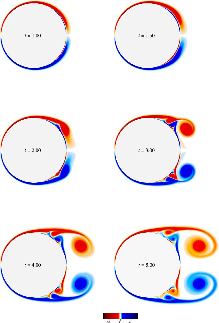
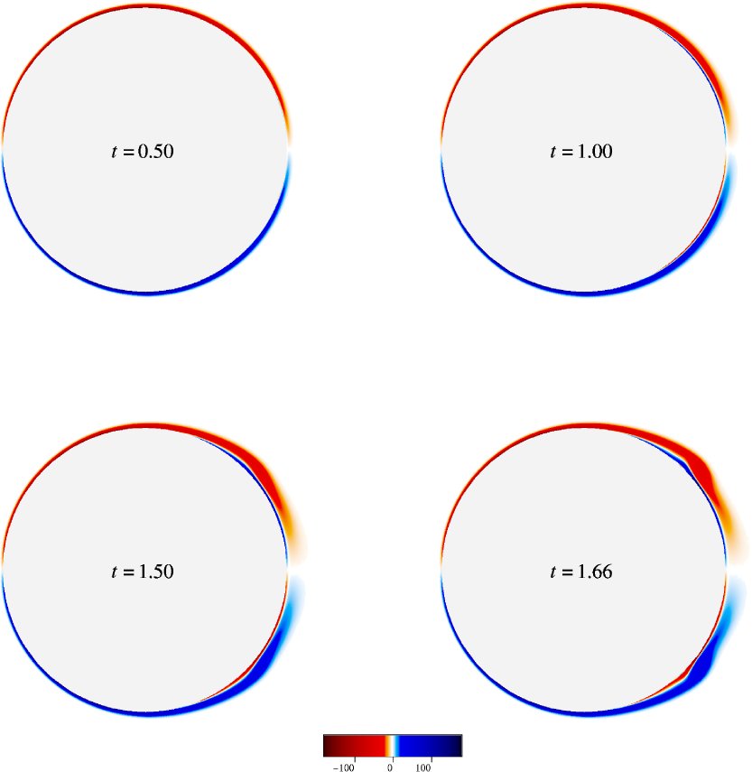
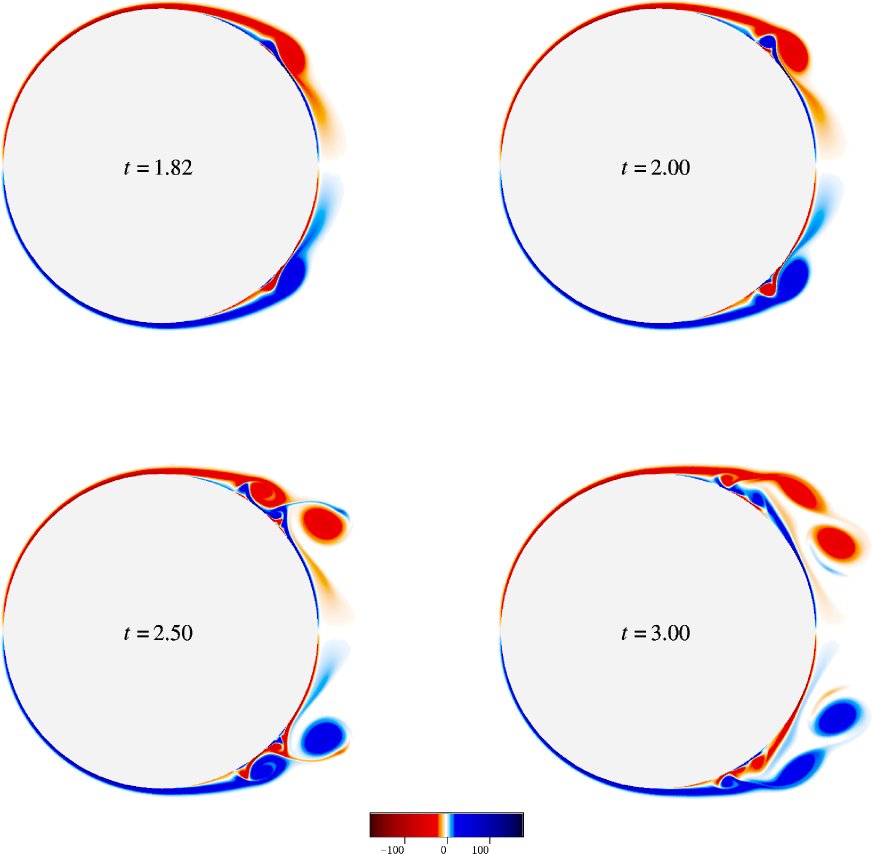
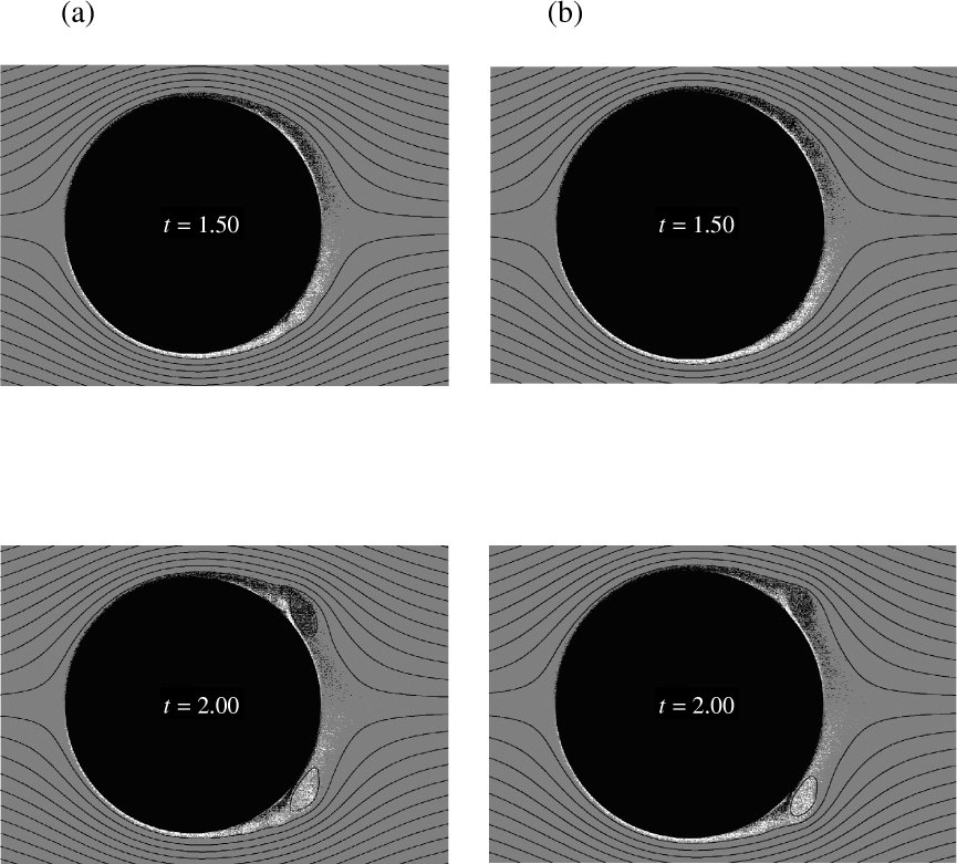
At later times, the boundary layer vorticity ``rolls up" or
``individualizes" into two discrete vortices at the rear half of the cylinder.
This is particularly clear at the higher Reynolds numbers
(figures 8.18 and 8.19).
It is believed to be the final result of an earlier ``Van Dommelen &
Shen" process, which turns the upper part of the boundary layer into a
free vortex sheet [242].
Such separation of vorticity layers from solid walls
has important consequences for flow control; for example, for dynamic
stall control of aircraft wings. This was investigated by
Shih, Lourenco, Van Dommelen, & Krothapalli [213].
Wang [245] studied flow control techniques that can prevent it.
when the cylinder has
moved a distance of one radius, the flow
at the rear surface of the cylinder is in the upstream direction.
This upstream flow (or flow
reversal) is indicated by a vorticity sublayer of opposite sign
(color in the figures)
to that of
the main boundary layer above it.
At later times, the boundary layer vorticity ``rolls up" or
``individualizes" into two discrete vortices at the rear half of the cylinder.
This is particularly clear at the higher Reynolds numbers
(figures 8.18 and 8.19).
It is believed to be the final result of an earlier ``Van Dommelen &
Shen" process, which turns the upper part of the boundary layer into a
free vortex sheet [242].
Such separation of vorticity layers from solid walls
has important consequences for flow control; for example, for dynamic
stall control of aircraft wings. This was investigated by
Shih, Lourenco, Van Dommelen, & Krothapalli [213].
Wang [245] studied flow control techniques that can prevent it.
In the following, we compare our vorticity fields to data obtained from experiments and other computations.
 |
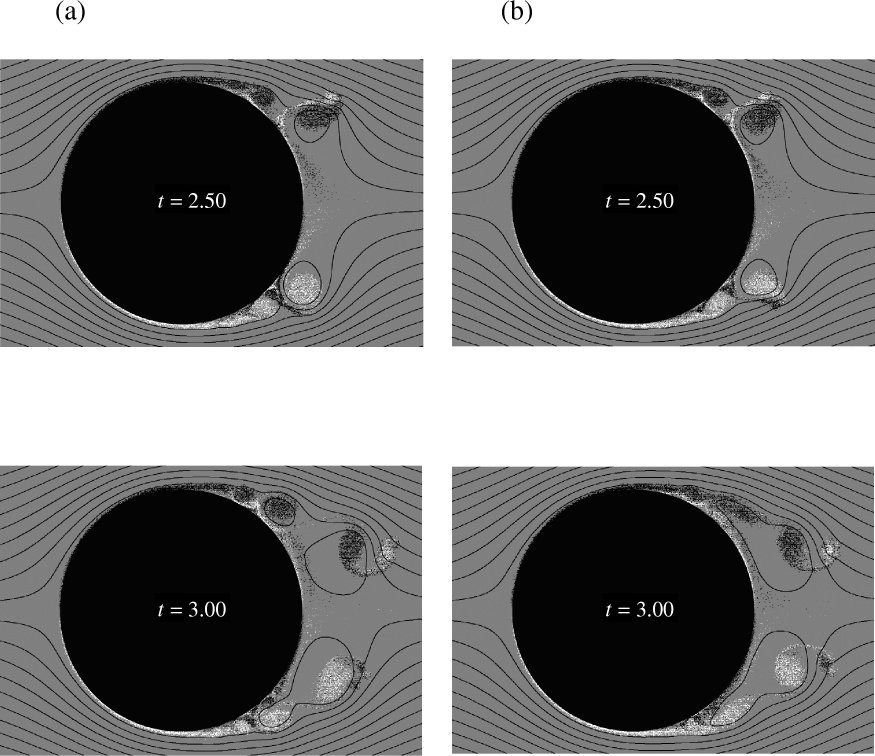
For example, we compare our computed vorticity fields for ![]() in figure 8.20 with the experimental results of
Shih, Lourenco & Ding [212].
We may point out that it has only become possible quite recently to
experimentally determine vorticity fields such as in figure
8.20.
The vorticity fields obtained from the experiment
in figure 8.20(a)
are evaluated by differentiating velocity
fields obtained
using the Particle Image Velocimetry (PIV) technique [136].
Plotted on exactly the same scale, our
computed vorticity fields are in excellent agreement with these
experimental results. Note the experimental perturbations
that tend to be smoothed out in less sensitive integrated quantities
such as the velocity field and even more in the streamlines. It shows
the sensitivity of the vorticity field as a basis of comparison of results.
in figure 8.20 with the experimental results of
Shih, Lourenco & Ding [212].
We may point out that it has only become possible quite recently to
experimentally determine vorticity fields such as in figure
8.20.
The vorticity fields obtained from the experiment
in figure 8.20(a)
are evaluated by differentiating velocity
fields obtained
using the Particle Image Velocimetry (PIV) technique [136].
Plotted on exactly the same scale, our
computed vorticity fields are in excellent agreement with these
experimental results. Note the experimental perturbations
that tend to be smoothed out in less sensitive integrated quantities
such as the velocity field and even more in the streamlines. It shows
the sensitivity of the vorticity field as a basis of comparison of results.
 |
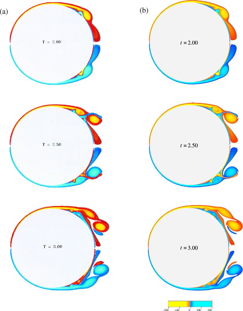 |
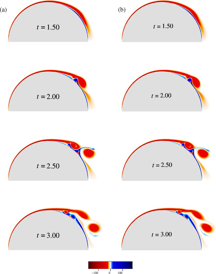
For Reynolds number ![]() , our computed vorticity
fields in figure 8.18
are in very good agreement with the high resolution
results of Kruse & Fischer using spectral element method
(figure 8.21)
and of Koumoutsakos & Leonard [117] using a vortex method
based on the Particle Strength Exchange scheme
(figure 8.22, different color scale from
figure 8.21).
This provides strong support for our results.
, our computed vorticity
fields in figure 8.18
are in very good agreement with the high resolution
results of Kruse & Fischer using spectral element method
(figure 8.21)
and of Koumoutsakos & Leonard [117] using a vortex method
based on the Particle Strength Exchange scheme
(figure 8.22, different color scale from
figure 8.21).
This provides strong support for our results.
 |
Our computed vorticity fields also agree quite well with the vorticity contours obtained from the high resolution finite difference computations of Anderson & Reider [3], and are in reasonable agreement with the random walk results of Van Dommelen (figure 8.23). Note however, that the random walk results develop a considerable asymmetry between top and bottom. Since the solution of the Navier-Stokes equations is unique, it must be symmetric; hence, the asymmetry in the random walk results is due to numerical errors. The fact that our present computation (figure 8.18) produces symmetric results although the scheme itself is not symmetric provides additional support for the correctness of our results.
The final issue is of course the remaining small differences in the vorticity fields of the most accurate three computations. Although both the spectral element computation of Kruse & Fischer, and the particle scheme of Koumoutsakos & Leonard used much more computational points than we did, still we have good reason to believe that ours may in fact be the most accurate of the three. In part, our reason is numerical convergence studies as found in figures 8.33(b) and 8.34(b). However, we also have good reasons to believe that in the past computations have been too optimistic about the levels of vorticity that they neglected. We postpone a full discussion to subsection 8.2.6. Here we merely note that regardless of the source, the differences in the vorticity fields between the best three computations are in any case very minor and our scheme is fully verified.
For practical applications, the most important result are the forces exerted on the cylinder. The lift force on the cylinder vanishes due to flow symmetry. We will examine the drag force in the next subsection.