A Simple Experiment on Process Dynamics
Introduction
Process dynamics is concerned with analyzing the time-dependent behavior of a process in response to an input change. Understanding the dynamic behavior is essential for process design, selection of optimal operating conditions, and for implementing process control strategies. However, a majority of experiments in a typical unit operations laboratory focus on the steady-state behavior of chemical processes.In this experiment, we analyze the dynamic behavior of a second-order system. The experiment is easy to perform; yet it requires the student to combine analytical as well as computational skills to analyze experimental data.
Experimental Set-up
A schematic of the experimental set-up is shown in Figure 1. There are two tanks connected in series. Each tank has a cross sectional area of 48.65 cm2. Water is fed to Tank 1 from an overhead reservoir. The reservoir has an overflow pipe near the top and is continuously supplied with water. The overflow pipe ensures that a constant flow rate is maintained at the inlet of the first tank. A strip of masking tape is attached to the side of each tank so that the water level at any given time can be marked off on the tape. The flow rates to the first tank and the second tank can be adjusted by ball valves. Initially, the water levels in the two tanks are at steady state. The objective of the experiment is to predict how the water level in the two tanks changes with time when a beaker full of water is suddenly added to the the first tank, and to verify this prediction experimentally.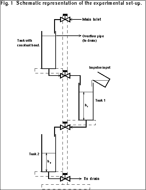
Theory
Assuming that:- the cross sectional area of both tanks is uniform and equal to A
- the density of water is constant

where qin and q1 are the volumetric flow rates of the inlet and outlet streams of Tank 1 and q2 is the volumetric flow rate of the outlet stream of Tank 2. The flow rates in the exit lines of the two tanks depend on the pressure drop, which in turn depend on the water levels h1 and h2 in the two tanks.
Linear Model
If a linear head-flow relationship is assumed, we get:
where R1 and R2 are the flow resistance terms of the pipes exiting from Tank 1 and Tank 2 respectively. Substituting, equation (2) in equation (1), and putting in matrix form, we get
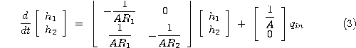
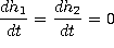
At steady state,
Thus, from equation (3):

where h1s and h2s are the steady state values of the water level in
Tank 1 and Tank 2 respectively and qins is the steady state flow rate.
It can be easily shown [1] that when qins is subjected to an impulse change
of strength M, and  , the impulse response is given by:
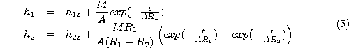
Equation (5) provides analytical expressions which predict the water levels h1 and h2 with time.
Nonlinear Model
The valve discharge rate in each tank can be modeled by the following square root law [2]:
where C1 and C2 are the valve coefficients of valves 1 and 2 respectively and depend on the valve openings. Substituting equation (6) in equation (1), the following nonlinear model is obtained:

At steady state,  .
Thus, from equation (7):
.
Thus, from equation (7):

When a beaker of water of volume M is suddenly added to Tank 1, the initial conditions of the system represented by equation (7) are given by:

The nonlinear model represented by equation (7) can be integrated numerically using the initial conditions given by equation (9) to predict how the water level in the two tanks changes with time.
Experimental Procedure
- Set up the apparatus as shown in Figure 1.
- Start the flow rate of water into the reservoir and wait till steady state is reached. Note the area of cross section of the two tanks.
- Measure the steady state heights in the two tanks.
- Measure the steady state flow rate of water coming out of the second tank with the help of a graduated cylinder and stop watch.
- Take a beaker of water (about 400 ml) and measure the volume of water in a graduated cylinder. Add this beaker of water to the first tank. At the same time, start the stop watch and mark off the level of water in both tanks.
- Mark off the level of water in both tanks in 10 second intervals for 120 seconds.
- Measure the water level recorded with time on the masking tape attached to each tank.
- Plot the water level in each tank versus time.
- Using the steady state values of the water level in each tank and the steady state flow rate, calculate the flow resistance R1 and R2, in the linear model using equation (4).
- Plot the analytical solution given by equation (5) on the same graph as the experimental data.
- Using the steady state values of the water level in each tank and the steady state flow rate, calculate the valve coefficients C1 and C2 in the nonlinear model using equation (8).
- Integrate the nonlinear model numerically in MATLAB [3] using the initial conditions given in equation (9).
- Plot the numerical solution given of the nonlinear model on the same graph as the experimental data.
- Comment on the accuracy of the linear model and the nonlinear model. Which is more accurate and why ?
Additional Problems
- The derivation of equation (5) assumes that
 . Under
what physical conditons would R1 = R2 ? Derive the impulse response
when R1 = R2.
. Under
what physical conditons would R1 = R2 ? Derive the impulse response
when R1 = R2.
- For what magnitude of the impulse input M is the linear model prediction close to the nonlinear model prediction ?
Nomenclature
| A | = | area of cross section of Tank 1 and Tank 2, cm2 |
| C1 | = | valve coefficient of Valve 1 |
| C2 | = | valve coefficient of Valve 2 |
| h1 | = | water level in Tank 1, cm |
| h2 | = | water level in Tank 2, cm |
| qin | = | volumetric flow rate into Tank 1, cm3/sec |
| q1 | = | volumetric flow rate out of Tank 1, cm3/sec |
| q2 | = | volumetric flow rate out of Tank 2, cm3/sec |
| R1 | = | flow resistance of Pipe 1 |
| R2 | = | flow resistance of Pipe 2 |
| t | = | time, sec |
References
- Seborg, D. E., Edgar, T. F., Mellichamp, D. A., Process Dynamics and Control, John Wiley and Sons, New York, 1989
- Perry, R. H., Chilton, C. H. Chemical Engineers' Handbook, 5th ed., McGraw Hill, New York, 1973
- MATLABTM, The Mathworks, Inc., Cochituate Place, South Natick, MA, USA