Chapter 2

Motion of a Point

1.

To design a vehicle, an engineer must be able to $\rule{1.0in}{.01in}$ and $\rule{1.0in}{.01in}$ its motion.

2.

In this chapter we are not concerned with the $\rule{1.0in}{.01in}$ of motion. We merely want to $\rule{1.0in}{.01in}$ and $\rule{1.0in}{.01in}$ the motion of a point in space.

3.

For a moving object this point might be the $\rule{1.0in}{.01in}$ $\rule{0.4in}{.01in}$ $\rule{1.0in}{.01in}$.

4.

Another name for path is $\rule{1.0in}{.01in}$.

5.

Important. Always (in your notes and completion of the reading journal) denote vectors by an overbar, e.g., ${\bar r}$. In the book vectors are denoted by only bold, e.g., ${\bf r}$, whereas in this reading journal vectors are denoted by both bold and an overbar, e.g., $\mbox{$\bar{{\bf r}}$}$.

Position, Velocity, and Accleration

1.

Sketch Figure 2.1(a) and (b) below.

2.

It is assumed that $\mbox{$\bar{{\bf r}}$}(t)$ is the position vector from O to P. Write a simple expression for $\mbox{$\bar{{\bf v}}$}$, the velocity of P relative to O at time t. (Your answer should be in terms of a derivative.)

3.

Write the definition of a derivative $\frac{d\mbox{$\bar{{\bf s}}$}}{dt}$ of a vector $\mbox{$\bar{{\bf s}}$}(t)$.

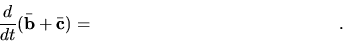
4.

Suppose $\mbox{$\bar{{\bf b}}$}$ and $\mbox{$\bar{{\bf c}}$}$ are vector functions of time (i.e., $\mbox{$\bar{{\bf b}}$}= \mbox{$\bar{{\bf b}}$}(t)$ and $\mbox{$\bar{{\bf c}}$}= \mbox{$\bar{{\bf c}}$}(t)$). Fill in the right hand side of the following:

$$\frac{d}{dt}(\mbox{$\bar{{\bf b}}$}+\mbox{$\bar{{\bf c}}$})=~~~~~~~~~~~~~~~~~~~~~~~~~~~~~~~~~~~~~~~~~~.$$

5.

Suppose $\gamma$ is a scalar function of time (i.e., $\gamma = \gamma(t)$) and $\mbox{$\bar{{\bf b}}$}$ is a vector function of time (i.e., $\mbox{$\bar{{\bf b}}$}= \mbox{$\bar{{\bf b}}$}(t)$). Fill in the right hand side of the following:

$$\frac{d(\gamma\mbox{$\bar{{\bf b}}$})}{dt}=~~~~~~~~~~~~~~~~~~~~~~~~~~~~~~~~~~~~~~~~~~.$$

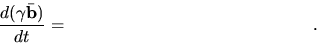
6.

Write a simple expression for $\mbox{$\bar{{\bf a}}$}$, the acceleration of P relative to O at time t. (Your answer should be in terms of a derivative.)

7.

Important. In this class scalars and vectors are often functions of time but this dependence is not explicitly recognized. You must learn to recognize (from the context) when a quantity is a function of time.

8.

Important. In this class scalars and vectors are often functions of time but this dependence is not explicitly recognized. You must learn to recognize (from the context) when a quantity is a function of time. (This repeat is not a typo.)

Straight-Line Motion

1.

List at least four examples of straight line motion.

Description of the Motion

1.

Sketch Figure 2.3(a) and (b) below (side-by-side). Important: Here and everywhere below, denote the unit vector by $\mbox{$\bf{\hat e}$}$ although the book does not use the ``hat''. (Of course, you can only use the hat and not the bold.)

2.

Fill in the right hand side of the following equations, following the book exactly. (However, unlike the book, denote the unit vector by $\mbox{$\bf{\hat e}$}$.)

Make sure that you understand each of the above steps!

3.

For straight line motion, the reason we can represent the position, velocity and acceleration by the scalars s, v and a is that the position vector, the velocity vector, and the acceleration vector are each in the direction described by the unit vector $\rule{0.5in}{.01in}$.

4.

Sketch Figures 2.4 and 2.5 below (side-by-side).

5.

Make sure that you understand the graphical interpretation of the derivative expressions for v(t) and a(t) as given by the above figures. That is, given a curve of s(t) can you compute (or at least estimate) v at a given time, and given a curve of v(t) can you compute or estimate a at a given time?

Analysis of the Motion

1.

Sketch Figure 2.6 below.

2.

Suppose t has units of seconds and

$$s = 5 + 2t^\frac{1}{2} m$$

Fill in the right hand side of the following equations. (Make sure you write the units.)

Acceleration Specified as a Function of Time

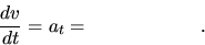
3.

Suppose that we know the acceleration a(t). Use indefinite integration to derive an expression for the velocity v. Label the equation for v ``(1)'' and denote the unknown constant by A.

4.

Now, suppose that we know the velocity v(t). Use indefinite integration to derive an expression for the position s. Label the equation for s ``(2)'' and denote the unknown constant by B.

5.

Describe the additional information we would need to determine the constants A and B in (1) and (2).

6.

Now, assume v(t₀)=v₀ and use definite integration to derive an expression for the velocity v. Label the equation for v ``(3)''.

7.

Assume s(t₀)=s₀ and use definite integration to derive an expression for the position s. Label the equation for s ``(4)''.

8.

Sketch Figures 2.7(a) and (b) below (side-by-side).

9.

Make sure that you understand the graphical interpretation of the integral expressions for v(t) and s(t) as given by the above figures. That is, given a graph of a(t), cay you compute or estimate v(t)-v(t₀) from this graph? Likewise, given a graph of v(t), can you compute or estimate s(t)-s(t₀) from this graph?

10.

If one neglects aerodynamic $\rule{1.0in}{.01in}$, then it can be assumed that an apple dropped from a tree at about sea level has constant acceleration.

11.

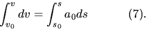
Assume that the acceleration a is a known constant a₀. Then, solve the integrals in (3) and (4) to obtain expressions for v and s as functions of time. Label these equations respectively ``(5)'' and ``(6)''.

12.

Use the chain rule to express the acceleration a (not necessarily constant) purely in terms of a derivative with respect to s.

13.

Fill in the missing step leading to the following integral expression.

$$\int_{v_0}^{v}dv = \int_{s_0}^{s}a_0 ds~~~~~~~~~~(7).$$

14.

Now assume that a is equal to the constant a₀. Integrate both sides of the above equation.

15.

Danger Will Robinson; Danger!! Equations (5) thru (7) are valid only when the acceleration is $\rule{1.0in}{.01in}$.

Curvilinear Motion

1.

For straight line motion, the position vector $\mbox{$\bar{{\bf r}}$}$, velocity vector $\mbox{$\bar{{\bf v}}$}$, and acceleration vector $\mbox{$\bar{{\bf a}}$}$ are described completely by the scalars s, v, and a respectively, since the directions of these vectors are parallel to a straight line. However, for curvilinear motion the direction of motion varies so we must be careful to describe both the $\rule{1.0in}{.01in}$ and $\rule{1.0in}{.01in}$ of these vectors.

Cartesian Coordinates

1.

Sketch Figure 2.15 below.

2.

Following the book, fill in the right hand side of the following equations.

$$\mbox{$\bar{{\bf v}}$}= ~~~~~~~~~~~~~~~~~.$$

$$\mbox{$\bar{{\bf v}}$}= ~~~~~~~~~~~~~~~~~.$$

$a_x=\rule{0.5in}{.01in}$,

$a_y=\rule{0.5in}{.01in}$,

$a_z=\rule{0.5in}{.01in}$.

Make sure that you understand each of the above steps.

3.

For a projectile problem in which the projectile moves in the x-y plane, $a_x=\rule{0.5in}{.01in}$, $a_y=\rule{0.5in}{.01in}$, and $a_z=\rule{0.5in}{.01in}$.

4.

Sketch Figure 2.16 below.

5.

Suppose the above figure describes the initial condition of a projectile. Derive an expressions for x and box in your final answer.

6.

Now, derive an expressions for y and box in your final answer.

7.

Using your above expressions for x and y, derive an expression for y as a function of x.

Angular Motion

Angular Motion of a Line

1.

Sketch Figure 2.18 below.

2.

The angular velocity $\omega$ of L relative to L₀ is defined by,

$$\omega = ~~~~~~~~~~~~~~~~~~~~~~.$$

3.

The angular acceleration $\alpha$ of L relative to L₀ is defined by,

$$\alpha = ~~~~~~~~~~~~~~~~~~~~~~.$$

4.

Write the contents of Table 2.2 below to enforce the fact that the equations of straight-line motion and angular motion are identical in form.

Straight-Line Motion     Angular Motion

Rotating Unit Vector

1.

Sketch Figure 2.19(a) below and at the tip of $\mbox{$\bf{\hat e}$}$ sketch the unit vector $\mbox{$\bf{\hat n}$}$.

2.

The unit vector $\mbox{$\bf{\hat n}$}$ is $\rule{1.0in}{.01in}$ to $\mbox{$\bf{\hat e}$}$ and points in the $\rule{2.0in}{.01in}$.

Normal and Tangential Components

1.

Sketch Figure 2.22 below.

2.

The unit vector $\mbox{${\bf{\hat e}}_t$}$ is $\rule{1.0in}{.01in}$ to the path in the direction of motion.

3.

The unit vectors $\mbox{${\bf{\hat e}}_t$}$ and $\mbox{${\bf{\hat e}}_n$}$ correspond respectively to $\mbox{$\bf{\hat e}$}$ and $\mbox{$\bf{\hat n}$}$ above (under the heading ``Rotating Unit Vector''). Hence, $\mbox{${\bf{\hat e}}_n$}$ is $\rule{1.0in}{.01in}$ to $\mbox{${\bf{\hat e}}_t$}$ and is in the positive $\theta$ direction.

4.

Write the expression for the velocity vector of P in terms of v and $\mbox{${\bf{\hat e}}_t$}$.

5.

Sketch Figure 2.24 below.

6.

Referring to the above figure, the instantaneous radius of curvature is the distance $\rule{0.4in}{.01in}$.

7.

Write the expression for the acceleration vector of P in terms of v, $\rho$, $\mbox{${\bf{\hat e}}_t$}$, and $\mbox{${\bf{\hat e}}_n$}$.

8.

Summarize the results by rewriting equations (2.38) thru (2.40) below.

Circular Motion

Sketch Figure 2.27 below.

Following the book complete the following equations.

Polar and Cylindrical Coordinates

1.

Sketch Figure 2.31(a) and (b) below (side-by-side).

2.

Write the expression for the position vector $\mbox{$\bar{{\bf r}}$}$ in terms of r and $\mbox{${\bf{\hat e}}_r$}$.

3.

Now, differentiate this expression for $\mbox{$\bar{{\bf r}}$}$ and use the fact that $\frac{d\mbox{${\bf{\hat e}}_r$}}{dt}=\omega\mbox{${\bf{\hat e}}_{\theta}$}$ to derive an expression for the velocity vector $\mbox{$\bar{{\bf v}}$}$ in terms of r, $\omega$, $\mbox{${\bf{\hat e}}_r$}$, and $\mbox{${\bf{\hat e}}_{\theta}$}$.

4.

Next, differentiate the expression for $\mbox{$\bar{{\bf v}}$}$, and use the additional facts that $\frac{d\mbox{${\bf{\hat e}}_{\theta}$}}{dt}=-\omega\mbox{${\bf{\hat e}}_r$}$ and $\alpha=\frac{d\omega}{dt}$ to derive an expression for the acceleration vector $\mbox{$\bar{{\bf a}}$}$ in terms of r, v, $\omega$, $\alpha$, $\mbox{${\bf{\hat e}}_r$}$, and $\mbox{${\bf{\hat e}}_{\theta}$}$. Express your final answer in the form $\mbox{$\bar{{\bf a}}$}= (\cdot)\mbox{${\bf{\hat e}}_r$}+ (\cdot)\mbox{${\bf{\hat e}}_{\theta}$}$.

5.

Summarize this subsection by writing equations (2.49) thru (2.51) below.

Circular Motion

Sketch Figures 2.35(a) and (b) below (side-by-side).

Write $\mbox{${\bf{\hat e}}_r$}$ in terms of $\mbox{${\bf{\hat e}}_n$}$ and $\mbox{${\bf{\hat e}}_{\theta}$}$ in terms of $\mbox{${\bf{\hat e}}_t$}$.

For circular motion, r is equal to the constant R. Hence the velocity expression in polar coordinates becomes,

$$\mbox{$\bar{{\bf v}}$}= ~~~~~~~~~~~~~~~~~.$$

In normal and tangential components, the velocity vector is $\mbox{$\bar{{\bf v}}$}=v\mbox{${\bf{\hat e}}_t$}$. Hence, comparing these two expressions for $\mbox{$\bar{{\bf v}}$}$ (and using equations $(\star)$ and $(\star\star)$), an expression for v in terms of R and $\omega$ is

v =                            .

For circular motion, the acceleration expression in polar coordinates becomes,

$$\mbox{$\bar{{\bf a}}$}= ~~~~~~~~~~~~~~~~~~~~~~~~~~~.$$

In normal and tangential components, the acceleration vector is 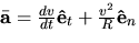$\mbox{$\bar{{\bf a}}$}=\frac{dv}{dt}\mbox{${\bf{\hat e}}_t$}+ \frac{v^2}{R}\mbox{${\bf{\hat e}}_n$}$. Hence, equating the transverse and tangential components of the two expressions for $\mbox{$\bar{{\bf a}}$}$ (and and using equations $(\star)$ and $(\star\star)$),

$$\frac{dv}{dt} = a_t = ~~~~~~~~~~~~~~~~~.$$

Cylindrical Coordinates

Polar coordinates describe the motion of a point P in $\rule{0.5in}{.01in}$ dimensional motion (i.e., in the x-y plane). Cylindrical coordinates are used to describe $\rule{1.0in}{.01in}$ dimensional motion.

Sketch Figure 2.36 below.

Summarize the formulas for cylindrical coordinates below by writing equations (2.52) thru (2.55) from the text.

The expression for $\mbox{$\bar{{\bf r}}$}$ in cylindrical coordinates differs from that for polar coordinates by the addition of the term $\rule{1.0in}{.01in}$. The expression for $\mbox{$\bar{{\bf v}}$}$ in cylindrical coordinates differs from that for polar coordinates by the addition of the term $\rule{1.0in}{.01in}$. The expression for $\mbox{$\bar{{\bf a}}$}$ in cylindrical coordinates differs from that for polar coordinates by the addition of the term $\rule{1.0in}{.01in}$.

Orbital Mechanics

This section may or may not be covered as will be mentioned in class.

Relative Motion

1.

Sketch Figure 2.46 below.

2.

Write $\mbox{$\bar{{\bf r}}$}_A$ in terms of $\mbox{$\bar{{\bf r}}$}_B$ and $\mbox{$\bar{{\bf r}}$}_{A/B}$.

3.

Differentiate the above expression to write $\mbox{$\bar{{\bf v}}$}_A$ in terms of $\mbox{$\bar{{\bf v}}$}_B$ and $\mbox{$\bar{{\bf v}}$}_{A/B}$.

4.

Differentiate the above expression to write $\mbox{$\bar{{\bf a}}$}_A$ in terms of $\mbox{$\bar{{\bf a}}$}_B$ and $\mbox{$\bar{{\bf a}}$}_{A/B}$.