| Quantum Mechanics for Engineers |
|
© Leon van Dommelen |
|
A.26 Fourier inversion theorem and Parseval
This note discusses Fourier series, Fourier integrals, and
Parseval’s identity.
Consider first one-dimensional Fourier series. They apply to functions
 that are periodic with some given period
  :
:
Such functions can be written as a “Fourier series:”
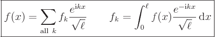 |
(A.193) |
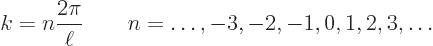
Here the  values are those for which the exponentials are periodic
of period . According to the Euler formula
(2.5), that means that
values are those for which the exponentials are periodic
of period . According to the Euler formula
(2.5), that means that  must be a whole multiple
  of
of  , so
, so
 |
(A.194) |
Note that notations for Fourier series can vary from one author to the
next. The above form of the Fourier series is the prefered one for
quantum mechanics. The reason is that the functions


 form an orthonormal set:
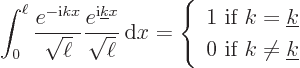 |
(A.195) |
Quantum mechanics just loves orthonormal sets of functions. In
particular, note that the above functions are momentum eigenfunctions.
Just apply the linear momentum operator 


 on them. That shows that their linear momentum
is given by the de Broglie relation
on them. That shows that their linear momentum
is given by the de Broglie relation 
 . Here
these momentum eigenfunctions are properly normalized. They would not
be using different conventions.
. Here
these momentum eigenfunctions are properly normalized. They would not
be using different conventions.
That any (reasonable) periodic function can be written as a
Fourier series was already shown in {D.8}. That
derivation took be the half-period. The formula for the
coefficients  can also be derived directly: simply multiply the
expression (A.193) for with
can also be derived directly: simply multiply the
expression (A.193) for with
 for any arbitrary value of
  and
integrate over
and
integrate over  . Because of the orthonormality
(A.195), the integration produces zero for all except if
, and then it produces
. Because of the orthonormality
(A.195), the integration produces zero for all except if
, and then it produces  as required.
Note from (A.193) that if you known you can find all the
. Conversely, if you know all the , you can
find at every position . The formulae work both ways.
But the symmetry goes even deeper than that. Consider the inner
product of a pair of functions and  :
:
Using the orthonormality property (A.195) that becomes
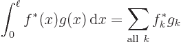 |
(A.196) |
Now note that if you look at the coefficients and  as the
coefficients of infinite-dimensional vectors, then the right
hand side is just the inner product of these vectors. In short,
Fourier series preserve inner products.
as the
coefficients of infinite-dimensional vectors, then the right
hand side is just the inner product of these vectors. In short,
Fourier series preserve inner products.
Therefore the equation above may be written more concisely as
 |
(A.197) |
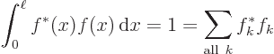
This is the so-called “Parseval identity.” Now transformations that preserve inner
products are called “unitary” in mathematics. So the Parseval identity shows that
the transformation from periodic functions to their Fourier
coefficients is unitary.
That is quite important for quantum mechanics. For example, assume
that is a wave function of a particle stuck on a ring of
circumference . Wave functions should be normalized, so:
According to the Born interpretation, the left hand side says that the
probability of finding the particle is 1, certainty, if you look at
every position on the ring. But according to the orthodox
interpretation of quantum mechanics,  in the right hand side
gives the probability of finding the particle with momentum
. The fact that the total sum is 1 means physically
that it is certain that the particle will be found with some
momentum.
in the right hand side
gives the probability of finding the particle with momentum
. The fact that the total sum is 1 means physically
that it is certain that the particle will be found with some
momentum.
So far, only periodic functions have been covered. But functions in
infinite space can be handled by taking the period infinite.
To do that, note from (A.194) that the values of the
Fourier series are spaced apart over a distance
In the limit  ,
,  becomes an
infinitesimal increment
becomes an
infinitesimal increment  , and the sums become integrals.
Now in quantum mechanics it is convenient to replace the coefficients
by a new function
, and the sums become integrals.
Now in quantum mechanics it is convenient to replace the coefficients
by a new function  that is defined so that
The reason that this is convenient is that  gives the
probability for wave number . Then for a function
that is defined as above,
gives the
probability for wave number . Then for a function
that is defined as above,  gives the probability per unit -range.
If the above definition and  are
substituted into the Fourier series expressions (A.193), in the
limit it gives the “Fourier integral” formulae:
are
substituted into the Fourier series expressions (A.193), in the
limit it gives the “Fourier integral” formulae:
 |
(A.198) |
In books on mathematics you will usually find function
indicated as  , to clarify that it is a
completely different function than . Unfortunately, the
hat is already used for something much more important in quantum
mechanics. So in quantum mechanics you will have to look at the
argument, or , to know which function it really is.
, to clarify that it is a
completely different function than . Unfortunately, the
hat is already used for something much more important in quantum
mechanics. So in quantum mechanics you will have to look at the
argument, or , to know which function it really is.
Of course, in quantum mechanics you are often more interested in the
momentum than in the wave number. So it is often convenient to define
a new function  so that
  gives the probability per
unit momentum range rather than unit wave number range. Because
, the needed rescaling of is by a factor
gives the probability per
unit momentum range rather than unit wave number range. Because
, the needed rescaling of is by a factor
 . That gives
 |
(A.199) |
Using similar substitutions as for the Fourier series, the Parseval
identity (A.197) becomes
or in short
 |
(A.200) |
This identity is sometimes called the “Plancherel theorem,” after a later mathematician who
generalized its applicability. The bottom line is that Fourier
integral transforms too conserve inner products.
So far, this was all one-dimensional. However, the extension to three
dimensions is straightforward. The first case to be considered is
that there is periodicity in each Cartesian direction:
In quantum mechanics, this would typically correspond to the wave
function of a particle stuck in a periodic box of dimensions 


 . When the particle leaves
such a box through one side, it reenters it at the same time through
the opposite side.
. When the particle leaves
such a box through one side, it reenters it at the same time through
the opposite side.
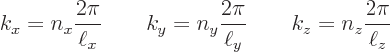
There are now wave numbers for each direction,
where  ,
,  , and
, and  are whole numbers. For
brevity, vector notations may be used:
are whole numbers. For
brevity, vector notations may be used:
Here  is the “wave number vector.”
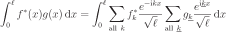
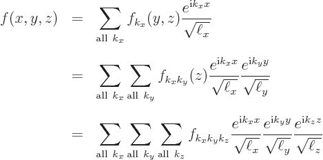
The Fourier series for a three-dimensional periodic function is
 |
(A.201) |
Here  is shorthand for
  and
and

 is the volume of the periodic box.
The above expression for  may be derived by applying the
one-dimensional transform in each direction in turn:
may be derived by applying the
one-dimensional transform in each direction in turn:
This is equivalent to what is given above, except for trivial changes
in notation. The expression for the Fourier coefficients can be
derived analogous to the one-dimensional case, integrating now over the
entire periodic box.
The Parseval equality still applies
 |
(A.202) |
where the left inner product integration is over the periodic box.
For infinite space
 |
(A.203) |
 |
(A.204) |
 |
(A.205) |
These expressions are all obtained completely analogously to the
one-dimensional case.
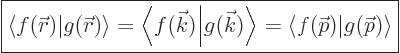
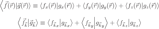
Often, the function is a vector rather than a scalar. That does not
make a real difference since each component transforms the same way.
Just put a vector symbol over and  in the above formulae.
The inner products are now defined as
in the above formulae.
The inner products are now defined as
For the picky, converting Fourier series into Fourier integrals only
works for well-behaved functions. But to show that it also works for
nasty wave functions, you can set up a limiting process in which you
approximate the nasty functions increasingly accurately using
well-behaved ones. Now if the well-behaved functions are converging,
then their Fourier transforms are too. The inner products of the
differences in functions are the same according to Parseval. And
according to the abstract Lebesgue variant of the theory of
integration, that is enough to ensure that the transform of the nasty
function exists. This works as long as the nasty wave function is
square integrable. And wave functions need to be in quantum
mechanics.
But being square integrable is not a strict requirement, as you may
have been told elsewhere. A lot of functions that are not square
integrable have meaningful, invertible Fourier transforms. For
example, functions whose square magnitude integrals are infinite, but
absolute value integrals are finite can still be meaningfully
transformed. That is more or less the classical version of the
inversion theorem, in fact. (See D.C. Champeney, A Handbook of
Fourier Theorems, for more.)