7.5 Symmetric Two-State Systems

This section will look at the simplest quantum systems that can have nontrivial time variation. They are called symmetric two-state systems. Despite their simplicity, a lot can be learned from them.

Symmetric two-state systems were encountered before in chapter 5.3. They describe such systems as the hydrogen molecule and molecular ion, chemical bonds, and ammonia. This section will show that they can also be used as a model for the fundamental forces of nature. And for the spontaneous emission of radiation by say excited atoms or atomic nuclei.

Two-state systems are characterized by just two basic states; these states will be called $\psi_1$ and $\psi_2$ . For symmetric two-state systems, these two states must be physically equivalent. Or at least they must have the same expectation energy. And the Hamiltonian must be independent of time.

For example, for the hydrogen molecular ion $\psi_1$ is the state where the electron is in the ground state around the first proton. And $\psi_2$ is the state in which it is in the ground state around the second proton. Since the two protons are identical in their properties, there is no physical difference between the two states. So they have the same expectation energy.

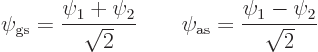
The interesting quantum mechanics arises from the fact that the two states $\psi_1$ and $\psi_2$ are not energy eigenstates. The ground state of the system, call it $\psi_{\rm {gs}}$ , is a symmetric combination of the two states. And there is also an excited energy eigenstate $\psi_{\rm {as}}$ that is an antisymmetric combination, chapter 5.3, {N.11}:

$\begin{displaymath} \psi_{\rm {gs}} = \frac{\psi_1+\psi_2}{\sqrt2} \qquad \psi_{\rm {as}} = \frac{\psi_1-\psi_2}{\sqrt2} \end{displaymath}$

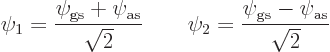
The above expressions may be inverted to give the states $\psi_1$ and $\psi_2$ in terms of the energy states:

$\begin{displaymath} \psi_1 = \frac{\psi_{\rm {gs}}+\psi_{\rm {as}}}{\sqrt2} \qquad \psi_2 = \frac{\psi_{\rm {gs}}-\psi_{\rm {as}}}{\sqrt2} \end{displaymath}$

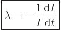
That makes their expectation energy $\langle{E}\rangle$ equal to the average of the two energies, and their uncertainty in energy $\Delta{E}$ equal to half the difference:

$\begin{displaymath} \langle{E}\rangle = \frac{E_{\rm {gs}}+E_{\rm {as}}}{2} \qquad \Delta E = \frac{E_{\rm {as}}-E_{\rm {gs}}}{2} \end{displaymath}$

The question in this section is how the system evolves in time. In general the wave function is, section 7.1,

$\begin{displaymath} \Psi = c_{\rm {gs}} e^{-{\rm i}E_{\rm {gs}} t/\hbar} \psi_... ... c_{\rm {as}} e^{-{\rm i}E_{\rm {as}} t/\hbar} \psi_{\rm {as}} \end{displaymath}$

However, this section will be more concerned with what happens to the basic states $\psi_1$ and $\psi_2$ , rather than to the energy eigenstates. So, it is desirable to rewrite the wave function above in terms of $\psi_1$ and $\psi_2$ and their properties. That produces:

$\begin{displaymath} \Psi = e^{-{\rm i}\langle E \rangle t/\hbar} \left[ c_{\r... ...rm i}\Delta E t/\hbar} \frac{\psi_1 - \psi_2}{\sqrt2} \right] \end{displaymath}$

$\begin{displaymath} \Psi = c_1 \psi_1 + c_2 \psi_2 \end{displaymath}$

The most interesting case is the one in which the system is in the state $\psi_1$ at time zero. In that case the probabilities of the states $\psi_1$ and $\psi_2$ vary with time as

$\begin{displaymath} \fbox{$\displaystyle \vert c_1\vert^2 = \cos^2(\Delta E ... ...) \qquad \vert c_2\vert^2 = \sin^2(\Delta E t/\hbar) $} % \end{displaymath}$

(7.27)

At time zero, the above probabilities produce state $\psi_1$ with 100% probability as they should. And so they do whenever the sine in the second expressions is zero. However, at times at which the cosine is zero, the system is fully in state $\psi_2$ . It follows that the system is oscillating between the states $\psi_1$ and $\psi_2$ .

7.5.1 A graphical example

Consider a simple example of the oscillatory behavior of symmetric two-state systems. The example system is the particle inside a closed pipe as discussed in chapter 3.5. It will be assumed that the wave function is of the form

$\begin{displaymath} \Psi=\sqrt{{\textstyle\frac{4}{5}}} e^{-{\rm i}E_{111}t/\hb... ...{\textstyle\frac{1}{5}}} e^{-{\rm i}E_{211}t/\hbar} \psi_{211} \end{displaymath}$

The above wave function is a valid solution of the Schrödinger equation since the two terms have the correct exponential dependence on time. And since the two terms have different energies, there is uncertainty in energy.

The relative probability to find the particle at a given position is given by the square magnitude of the wave function. That works out to

$\begin{displaymath} \vert\Psi\vert^2=\Psi^*\Psi = {\textstyle\frac{4}{5}} \ver... ...1}\psi_{211} + {\textstyle\frac{1}{5}} \vert\psi_{211}\vert^2 \end{displaymath}$

**Figure 7.6:** A combination of two energy eigenfunctions seen at some typical times.
Move your mouse over any figure to see the animation. Javascript must be enabled on your browser. Give it a few seconds for the animation to load, especially on a phone line.

The probability for finding the particle is plotted at four representative times in figure 7.6. After time (d) the evolution repeats at (a). The wave function blob is sloshing back and forth in the pipe. That is much like a classical frictionless particle with kinetic energy would bounce back and forth between the ends of the pipe.

In terms of symmetric two-state systems, you can take the state $\psi_1$ to be the one in which the blob is at its leftmost position, figure 7.6(a). Then $\psi_2$ is the state in which the blob is at its rightmost position, figure 7.6(c). Note from the figure that these two states are physically equivalent. And they have uncertainty in energy.

7.5.2 Particle exchange and forces

An important two-state system very similar to the simple example in the previous subsection is the hydrogen molecular ion. This ion consists of two protons and one electron.

The molecular ion can show oscillatory behavior very similar to that of the example. In particular, assume that the electron is initially in the ground state around the first proton, corresponding to state $\psi_1$ . In that case, after some time interval $\Delta{t}$ , the electron will be found in the ground state around the second proton, corresponding to state $\psi_2$ . After another time interval $\Delta{t}$ , the electron will be back around the first proton, and the cycle repeats. In effect, the two protons play catch with the electron!

That may be fun, but there is something more serious that can be learned. As is, there is no (significant) force between the two protons. However, there is a second similar play-catch solution in which the electron is initially around the second proton instead of around the first. If these two solutions are symmetrically combined, the result is the ground state of the molecular ion. In this state of lowered energy, the protons are bound together. In other words, there is now a force that holds the two protons together:

A play catch mechanism as described above is used in more advanced quantum mechanics to explain the forces of nature. For example, consider the correct, relativistic, description of electromagnetism, given by “quantum electrodynamics”. In it, the electromagnetic interaction between two charged particles comes about largely through processes in which one particle creates a photon that the other particle absorbs and vice versa. Charged particles play catch using photons.

That is much like how the protons in the molecular ion get bound together by exchanging the electron. Note however that the solution for the ion was based on the Coulomb potential. This potential implies instantaneous interaction at a distance: if, say, the first proton is moved, the electron and the other proton notice this instantaneously in the force that they experience. Classical relativity, however, does not allow effects that propagate at infinite speed. The highest possible propagation speed is the speed of light. In classical electromagnetics, charged particles do not really interact instantaneously. Instead charged particles interact with the electromagnetic field at their location. The electromagnetic field then communicates this to the other charged particles, at the speed of light. The Coulomb potential is merely a simple approximation, for cases in which the particle velocities are much less than the speed of light.

In a relativistic quantum description, the electromagnetic field is quantized into photons. (A concise introduction to this advanced topic is in addendum {A.23}.) Photons are bosons with spin 1. Similarly to classical electrodynamics, in the quantum description charged particles interact with photons at their location. They do not interact directly with other charged particles.

These are three-particle interactions, a boson and two fermions. For example, if an electron absorbs a photon, the three particles involved are the photon, the electron before the absorption, and the electron after the absorption. (Since in relativistic applications particles may be created or destroyed, a particle after an interaction should be counted separately from an identical particle that may exist before it.)

The ideas of quantum electrodynamics trace back to the early days of quantum mechanics. Unfortunately, there was the practical problem that the computations came up with infinite values. A theory that got around this problem was formulated in 1948 independently by Julian Schwinger and Sin-Itiro Tomonaga. A different theory was proposed that same year by Richard Feynman based on a more pictorial approach. Freeman Dyson showed that the two theories were in fact equivalent. Feynman, Schwinger, and Tomonaga received the Nobel prize in 1965 for this work, Dyson was not included. (The Nobel prize in physics is limited to a maximum of three recipients.)

Following the ideas of quantum electrodynamics and pioneering work by Sheldon Glashow, Steven Weinberg and Abdus Salam in 1967 independently developed a particle exchange model for the so called “weak force.” All three received the Nobel prize for that work in 1979. Gerardus ’t Hooft and Martinus Veltman received the 1999 Nobel Prize for a final formulation of this theory that allows meaningful computations.

The weak force is responsible for the beta decay of atomic nuclei, among other things. It is of key importance for such nuclear reactions as the hydrogen fusion that keeps our sun going. In weak interactions, the exchanged particles are not photons, but one of three different bosons of spin 1: the negatively charged W $\POW9,{-}$ , (think W for weak force), the positively charged W $\POW9,{+}$ , and the neutral Z $\POW9,{0}$ (think Z for zero charge). You might call them the massives because they have a nonzero rest mass, unlike the photons of electromagnetic interactions. In fact, they have gigantic rest masses. The W $\POW9,{\pm}$ have an experimental rest mass energy of about 80 GeV (giga-electron-volt) and the Z $\POW9,{0}$ about 91 GeV. Compare that with the rest mass energy of a proton or neutron, less than a GeV, or an electron, less than a thousandth of a GeV. However, a memorable name like massives is of course completely unacceptable in physics. And neither would be weak-force carriers, because it is accurate and to the point. So physicists call them the “intermediate vector bosons.” That is also three words, but completely meaningless to most people and almost meaningless to the rest, {A.20}. It meets the requirements of physics well.

A typical weak interaction might involve the creation of say a W $\POW9,{-}$ by a quark inside a neutron and its absorption in the creation of an electron and an antineutrino. Now for massive particles like the intermediate vector bosons to be created out of nothing requires a gigantic quantum uncertainty in energy. Following the idea of the energy-time equality (7.9), such particles can only exist for extremely short times. And that makes the weak force of extremely short range.

The theory of “quantum chromedynamics” describes the so-called “strong force” or “color force.” This force is responsible for such things as keeping atomic nuclei together.

The color force acts between “quarks.” Quarks are the constituents of “baryons” like the proton and the neutron, and of “mesons” like the pions. In particular, baryons consist of three quarks, while mesons consist of a quark and an antiquark. For example, a proton consists of two so-called up quarks and a third down quark. Since up quarks have electric charge $\frac23e$ and down quarks $-\frac13e$ , the net charge of the proton $\frac23e+\frac23e-\frac13e$ equals

. Similarly, a neutron consists of one up quark and two down quarks. That makes its net charge $\frac23e-\frac13e-\frac13e$ equal to zero. As another example, a so-called $\pi^+$ meson consists of an up quark and an antidown quark. An antiparticle has the opposite charge from the corresponding particle, so the charge of the $\pi^+$ meson $\frac23e+\frac13e$ equals

, the same as the proton. Three antiquarks make up an antibaryon. That gives an antibaryon the opposite charge of the corresponding baryon. More exotic baryons and mesons may involve the strange, charm, bottom, and top flavors of quarks. (Yes, there are six of them. You might well ask, “Who ordered that?” as the physicist Rabi did in 1936 upon the discovery of the muon, a heavier version of the electron. He did not know the least of it.)

Quarks are fermions with spin $\leavevmode \kern.03em\raise.7ex\hbox{\the\scriptfont0 1}\kern-.2em /\kern-.21em\lower.56ex\hbox{\the\scriptfont0 2}\kern.05em$ like electrons. However, quarks have an additional property called “color charge.” (This color charge has nothing to do with the colors you can see. There are just a few superficial similarities. Physicists love to give complete different things identical names because it promotes such hilarious confusion.) There are three quark colors called, you guessed it, red, green and blue. There are also three corresponding anticolors called cyan, magenta, and yellow.

Now the electric charge of quarks can be observed, for example in the form of the charge of the proton. But their color charge cannot be observed in our macroscopic world. The reason is that quarks can only be found in colorless combinations. In particular, in baryons each of the three quarks takes a different color. (For comparison, on a video screen full-blast red, green and blue produces a colorless white.) Similarly, in antibaryons, each of the antiquarks takes on a different anticolor. In mesons the quark takes on a color and the antiquark the corresponding anticolor. (For example on a video screen, if you define antigreen as magenta, i.e. full-blast red plus blue, then green and antigreen produces again white.)

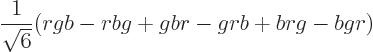
Actually, it is a bit more complicated still than that. If you had a green and magenta flag, you might call it color-balanced, but you would definitely not call it colorless. At least not in this book. Similarly, a green-antigreen meson would not be colorless, and such a meson does not exist. An actual meson is an quantum superposition of the three possibilities red-antired, green-antigreen, and blue-antiblue. The meson color state is

$\begin{displaymath} \frac{1}{\sqrt3}(r\bar r + g \bar g + b \bar b) \end{displaymath}$

In addition, the meson color state above is a one-of-a-kind, or “singlet” state. To see why, suppose that, say, the final $b\bar{b}$ term had a minus sign instead of a plus sign. Then surely, based on symmetry arguments, there should also be states where the $g\bar{g}$ or $r\bar{r}$ has the minus sign. And that cannot be true because linear combinations of such states would produce states like the green-antigreen meson that are not colorless. So the only true colorless possibility is the state above, where all three color-anticolor states have the same coefficient. (Do recall that a constant of magnitude one is indeterminate in quantum states. So if all three color-anticolor states had a minus sign, it would still be the same state.)

Similarly, an rgb baryon with the first quark red, the second green, and the third blue would be color-balanced but not colorless. So such a baryon does not exist. For baryons there are six different possible color combinations: there are three possibilities for which of the three quarks is red, times two possibilities which of the remaining two quarks is green. An actual baryon is a quantum superposition of these six possibilities. Moreover, the combination is antisymmetric under color exchange:

$\begin{displaymath} \frac{1}{\sqrt6}(rgb - rbg + gbr - grb + brg - bgr) \end{displaymath}$

It is believed that baryons and mesons cannot be taken apart into separate quarks to study quarks in isolation. In other words, quarks are subject to “confinement” inside colorless baryons and mesons. The problem with trying to take these apart is that the force between quarks does not become zero with distance like other forces. If you try to take a quark out of a baryon or meson, presumably eventually you will put in enough energy to create a quark-antiquark pair in between. That kills off the quark separation that you thought you had achieved.

The color force between quarks is due to the exchange of so-called “gluons.” Gluons are massless bosons with spin 1 like photons. However, photons do not carry electric charge. Gluons do carry color/anticolor combinations. That is one reason that quantum chromedynamics is enormously more difficult than quantum electrodynamics. Photons cannot move electric charge from one fermion to the next. But gluons allow the interchange of colors between quarks.

Also, because photons have no charge, they do not interact with other photons. But since gluons themselves carry color, gluons do interact with other gluons. In fact, both three-gluon and four-gluon interactions are possible. In principle, this makes it conceivable that “glueballs,” colorless combinations of gluons, might exist. However, at the time of writing, 2012, only baryons, antibaryons, and mesons have been solidly established.

Gluon-gluon interactions are related to an effective strengthening of the color force at larger distances. Or as physicists prefer to say, to an effective weakening of the interactions at short distances called “asymptotic freedom.” This helps a bit because it allows some analysis to be done at very short distances, i.e. at very high energies.

Normally you would expect nine independent color/anticolor gluon states: there are three colors times three anticolors. But in fact only eight independent gluon states are believed to exist. Recall the colorless meson state described above. If a gluon could be in such a colorless state, it would not be subject to confinement. It could then be exchanged between distant protons and neutrons, giving rise to a long-range nuclear force. Since such a force is not observed, it must be concluded that gluons cannot be in the colorless state. So if the nine independent orthonormal color states are taken to be the colorless state plus eight more states orthogonal to it, then only the latter eight states can be observable. In terms of section 7.3, the relevant symmetry of the color force must be SU(3), not U(3).

Many people contributed to the theory of quantum chromedynamics. However Murray Gell-Mann seemed to be involved in pretty much every stage. He received the 1969 Nobel Prize at least in part for his work on quantum chromedynamics. It is also he who came up with the name quark. The name is really not bad compared to many other terms in physics. However, Gell-Mann is also responsible for not spelling color” as “qolor. That would have saved countless feeble explanations that, “No, this color has absolutely nothing to do with the color that you see in nature.” So far nobody has been able to solve that problem, but David Gross, David Politzer and Frank Wilczek did manage to discover the asymptotic freedom mentioned above. For that they were awarded the 2004 Nobel Prize in Physics.

It may be noted that Gell-Mann initially called the three colors red, white, and blue. Just like the colors of the US flag, in short. Or of the Netherlands and Taiwan, to mention a few others. Huang, [27, p. 167], born in China, with a red and yellow flag, claims red, yellow and green are now the conventional choice. He must live in a world different from ours. Sorry, but the honor of having the color-balanced, (but not colorless), flag goes to Azerbaijan.

The force of gravity is supposedly due to the exchange of particles called “gravitons.” They should be massless bosons with spin 2. However, it is hard to experiment with gravity because of its weakness on human scales. The graviton remains unconfirmed. Worse, the exact place of gravity in quantum mechanics remains very controversial.

7.5.3 Spontaneous emission

Symmetric two state systems provide the simplest model for spontaneous emission of radiation by atoms or atomic nuclei. The general ideas are the same whether it is an atom or nucleus, and whether the radiation is electromagnetic (like visible light) or nuclear alpha or beta radiation. But to be specific, this subsection will use the example of an excited atomic state that decays to a lower energy state by releasing a photon of electromagnetic radiation. The conservation laws applicable to this process were discussed earlier in section 7.4. This subsection wants to examine the actual mechanics of the emission process.

First, there are some important terms and concepts that must be mentioned. You will encounter them all the time in decay processes.

The big thing is that decay processes are random. A typical atom in an excited state $\psi_{\rm {H}}$ will after some time transition to a state of lower energy $\psi_{\rm {L}}$ while releasing a photon. But if you take a second identical atom in the exact same excited state, the time after which this atom transitions will be different.

Still, the decay process is not completely unpredictable. Averages over large numbers of atoms have meaningful values. In particular, suppose that you have a very large number

of identical excited atoms. Then the “decay rate” is by definition

$\begin{displaymath} \fbox{$\displaystyle \lambda = - \frac{1}{I} \frac{{\rm d}I}{{\rm d}t} $} % \end{displaymath}$

(7.28)

To be precise, the above decay rate is better called the specific decay rate. The actual decay rate is usually defined to be simply $\vphantom{0}\raisebox{1.5pt}{$-$}$ ${\rm d}{I}$ $\raisebox{.5pt}{$/$}$ ${\rm d}{t}$ . But anyway, decay rate is not a good term to use in physics. It is much too clear. Sometimes the term “spontaneous emission rate” or “transition rate” is used, especially in the context of atoms. But that is even worse. A better and very popular choice is “decay constant.” But, while constant is a term that can mean anything, it really is still far too transparent. How does “disintegration constant” sound? Especially since the atom hardly disintegrates in the transition? Why not call it the [specific] “activity,” come to think of it? Activity is another of these vague terms. Another good one is “transition probability,” because a probability should be nondimensional and $\lambda$ is per unit time. May as well call it “radiation probability” then. Actually, many references will use a bunch of these terms interchangeably on the same page.

In fact, would it not be a good thing to take the inverse of the decay rate? That allows another term to be defined for essentially the same thing: the [mean] “lifetime” of the excited state:

$\begin{displaymath} \fbox{$\displaystyle \tau \equiv \frac{1}{\lambda} $} % \end{displaymath}$

(7.29)

Now suppose that initially there is a large number

of excited atoms. Then the number of excited atoms

left at a later time

$\begin{displaymath} \fbox{$\displaystyle I = I_0 e^{-\lambda t} $} % \end{displaymath}$

(7.30)

A quantity with a clearer physical meaning than lifetime is the time for about half the nuclei in a given large sample of excited atoms to decay. This time is called the “half-life” $\tau_{1/2}$ . From (7.30) and (7.29) above, it follow that the half-life is shorter than the lifetime by a factor $\ln2$ :

$\begin{displaymath} \fbox{$\displaystyle \tau_{1/2} = \tau \ln 2 $} % \end{displaymath}$

(7.31)

The purpose in this subsection is now to understand some of the above concepts in decays using the model of a symmetric two-state system.

The initial state $\psi_1$ of the system is taken to be an atom in a high-energy atomic state $\psi_{\rm {H}}$ , figure 7.3. The state seems to be an state of definite energy. That would make it a stationary state, section 7.1.4, and hence it would not decay. However, $\psi_1$ is not really an energy eigenstate, because an atom is always perturbed by a certain amount of ambient electromagnetic radiation. The actual state $\psi_1$ has therefore some uncertainty in energy $\Delta{E}$ .

The decayed state $\psi_2$ consists of an atomic state of lowered energy $\psi_{\rm {L}}$ plus an emitted photon. This state seems to have the same combined energy as the initial state $\psi_1$ . It too, however, is not really an energy eigenstate. Otherwise it would always have existed. In fact, it has the same expectation energy and uncertainty in energy as the initial state, section 7.1.3.

The probabilities of the two states were given at the start of this section. They were:

$\begin{displaymath} \vert c_1\vert^2 = \cos^2(\Delta E t/\hbar) \qquad \vert c_2\vert^2 = \sin^2(\Delta E t/\hbar) % \end{displaymath}$

(7.32)

$\begin{displaymath} \Delta t = {\textstyle\frac{1}{2}} \pi \hbar / \Delta E \end{displaymath}$

But note that there is a problem. According to (7.32), after another time interval $\Delta{t}$ the probabilities of the two states will revert back to the initial ones. That means that the low energy atomic state absorbs the photon again and so returns to the excited state!

Effects like that do occur in nuclear magnetic resonance, chapter 13.6, or for atoms in strong laser light and high vacuum, [52, pp. 147-152]. But normally, decayed atoms stay decayed.

To explain that, it must be assumed that the state of the system is measured according to the rules of quantum mechanics, chapter 3.4. The macroscopic surroundings observes that a photon is released well before the original state can be restored. In the presence of such significant interaction with the macroscopic surroundings, the two-state evolution as described above is no longer valid. In fact, the macroscopic surroundings will have become firmly committed to the fact that the photon has been emitted. Little chance for the atom to get it back under such conditions.

In an improved model of the transition process, section 7.6.1, the need for measurement remains. However, the reasons get more complex.

Interactions with the surroundings are generically called collisions. For example, a real-life atom in a gas will periodically collide with neighboring atoms and other particles. If a process is fast enough that no interactions with the surroundings occur during the time interval of interest, then the process takes place in the so-called “collisionless regime.” Nuclear magnetic resonance and atoms in strong laser light and high vacuum may be in this regime.

However, normal atomic decays take place in the so-called “collision-dominated regime.” Here collisions with the surroundings occur almost immediately.

To model that, take the time interval between collisions to be $t_{\rm {c}}$ . Assume that the atom evolves as an unperturbed two-state system until time $t_{\rm {c}}$ . At that time however, the atom is measured by its surroundings and it is either found to be in the initial excited state $\psi_1$ or in the decayed state with photon $\psi_2$ . According to the rules of quantum mechanics the result is random. However, they are not completely random. The probability $P_{1\to2}$ for the atom to be found to be decayed is the square magnitude $\vert c_2\vert^2$ of the state $\psi_2$ .

$\begin{displaymath} P_{1\to2} = \frac{\vert\Delta E\vert^2}{\hbar^2} t_{\rm {c}}^2 \end{displaymath}$

Note that the decay process has become probabilistic. You cannot say for sure whether the atom will be decayed or not at time $t_{\rm {c}}$ . You can only give the chances. See chapter 8.6 for a further discussion of that philosophical issue.

However, if you have not just one excited atom, but a large number

of them, then $P_{1\to2}$ above is the relative fraction that will be found to be decayed at time $t_{\rm {c}}$ . The remaining atoms, which are found to be in the excited state, (or rather, have been pushed back into the excited state), start from scratch. Then at time $2t_{\rm {c}}$ , a fraction $P_{1\to2}$ of these will be found to be decayed. And so on. Over time the number

of excited atoms decreases to zero.

As mentioned earlier, the relative fraction of excited atoms that disappears per unit time is called the decay rate $\lambda$ . That can be found by simply dividing the decay probability $P_{1\to2}$ above by the time $t_{\rm {c}}$ that the evolution took. So

$\begin{displaymath} \lambda_{1\to2} = \frac{\vert H_{21}\vert^2}{\hbar^2} t_{\r... ...uad H_{21}= \Delta E = \langle\psi_2\vert H\vert\psi_1\rangle. \end{displaymath}$

Physicists call $H_{21}$ the “matrix element.” That is well below their usual form, because it really is a matrix element. But before you start seriously doubting the capability of physicists to invariably come up with confusing terms, note that there are lots of different matrices in any advanced physical analysis. So the name does not give its secret away to nonspecialists. To enforce that, many physicists write matrix elements in the form $M_{21}$ , because, hey, the word matrix starts with an m. That hides the fact that it is an element of a Hamiltonian matrix pretty well.

The good news is that the assumption of collisions has solved the problem of decayed atoms undecaying again. Also, the decay process is now probabilistic. And the decay rate $\lambda_{1\to2}$ above is a normal number, not a random one.

Unfortunately, there are a couple of major new problems. One problem is that the state $\psi_2$ has one more particle than state $\psi_1$ ; the emitted photon. That makes it impossible to evaluate the matrix element using nonrelativistic quantum mechanics as covered in this book. Nonrelativistic quantum mechanics does not allow for new particles to be created or old ones to be destroyed. To evaluate the matrix element, you need relativistic quantum mechanics. Section 7.8 will eventually manage to work around that limitation using a dirty trick. Addendum {A.24} gives the actual relativistic derivation of the matrix element. However, to really understand that addendum, you may have to read a couple of others.

An even bigger problem is that the decay rate above is proportional to the collision time $t_{\rm {c}}$ . That makes it completely dependent on the details of the surroundings of the atom. But that is wrong. Atoms have very specific decay rates. These rates are the same under a wide variety of environmental conditions.

The basic problem is that in reality there is not just a single decay process for an excited atom; there are infinitely many. The derivation above assumed that the photon has an energy exactly given by the difference between the atomic states. However, there is uncertainty in energy one way or the other. Decays that produce photons whose frequency is ever so slightly different will occur too. To deal with that complication, asymmetric two-state systems must be considered. That is done in the next section.

Finally, a few words should probably be said about what collisions really are. Darn. Typically, they are pictured as atomic collisions. But that may be in a large part because atomic collisions are quite well understood from classical physics. Atomic collisions do occur, and definitely need to be taken into account, like later in the derivations of {D.41}. But in the above description, collisions take on a second role as doing quantum mechanical measurements. In that second role, a collision has occurred if the system has been measured to be in one state or the other. Following the analysis of chapter 8.6, measurement should be taken to mean that the surroundings has become firmly committed that the system has decayed. In principle, that does not require any actual collision with the atom; the surroundings could simply observe that the photon is present. The bad news is that the entire process of measurement is really not well understood at all. In any case, the bottom line to remember is that collisions do not necessarily represent what you would intuitively call collisions. Their dual role is to represent the typical moment that the surroundings commits itself that a transition has occurred.