| Quantum Mechanics for Engineers |
|
© Leon van Dommelen |
|
11.12 The New Variables
The new kid on the block is the entropy  . For an adiabatic
system the entropy is always increasing. That is highly useful
information, if you want to know what thermodynamically stable final
state an adiabatic system will settle down into. No need to try to
figure out the complicated time evolution leading to the final state.
Just find the state that has the highest possible entropy ,
that will be the stable final state.
. For an adiabatic
system the entropy is always increasing. That is highly useful
information, if you want to know what thermodynamically stable final
state an adiabatic system will settle down into. No need to try to
figure out the complicated time evolution leading to the final state.
Just find the state that has the highest possible entropy ,
that will be the stable final state.
But a lot of systems of interest are not well described as being
adiabatic. A typical alternative case might be a system in a rigid
box in an environment that is big enough, and conducts heat well
enough, that it can at all times be taken to be at the same
temperature  . Also assume that initially the
system itself is in some state 1 at the ambient temperature
, and that it ends up in a state 2 again at that
temperature. In the evolution from 1 to 2, however, the system
temperature could be be different from the surroundings, or even
undefined, no thermal equilibrium is assumed. The first law, energy
conservation, says that the heat
. Also assume that initially the
system itself is in some state 1 at the ambient temperature
, and that it ends up in a state 2 again at that
temperature. In the evolution from 1 to 2, however, the system
temperature could be be different from the surroundings, or even
undefined, no thermal equilibrium is assumed. The first law, energy
conservation, says that the heat  added to the system from the
surroundings equals the change in internal energy
added to the system from the
surroundings equals the change in internal energy  of the
system. Also, the entropy change in the isothermal environment will
be
of the
system. Also, the entropy change in the isothermal environment will
be 
 , so the system entropy change
 must be at least in order for the
net entropy in the universe not to decrease. From that it can be seen
by simply writing it out that the “Helmholtz free energy”
must be at least in order for the
net entropy in the universe not to decrease. From that it can be seen
by simply writing it out that the “Helmholtz free energy”
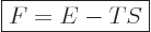 |
(11.21) |
is smaller for the final system 2 than for the starting one 1. In
particular, if the system ends up into a stable final state that can
no longer change, it will be the state of smallest possible Helmholtz
free energy. So, if you want to know what will be the final fate of a
system in a rigid, heat conducting, box in an isothermal environment,
just find the state of lowest possible Helmholtz energy. That will be
the one.
A slightly different version occurs even more often in real
applications. In these the system is not in a rigid box, but instead
its surface is at all times exposed to ambient atmospheric pressure.
Energy conservation now says that the heat added equals the
change in internal energy plus the work done
expanding against the atmospheric pressure, which is
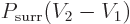 . Assuming that both the initial state
1 and final state 2 are at ambient atmospheric pressure, as well as at
ambient temperature as before, then it is seen that the quantity that
decreases is the “Gibbs free energy”
. Assuming that both the initial state
1 and final state 2 are at ambient atmospheric pressure, as well as at
ambient temperature as before, then it is seen that the quantity that
decreases is the “Gibbs free energy”
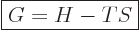 |
(11.22) |
in terms of the enthalpy  defined as
 . As an
example, phase equilibria are at the same pressure and temperature.
In order for them to be stable, the phases need to have the same
specific Gibbs energy. Otherwise all particles would end up in
whatever phase has the lower Gibbs energy. Similarly, chemical
equilibria are often posed at an ambient pressure and temperature.
. As an
example, phase equilibria are at the same pressure and temperature.
In order for them to be stable, the phases need to have the same
specific Gibbs energy. Otherwise all particles would end up in
whatever phase has the lower Gibbs energy. Similarly, chemical
equilibria are often posed at an ambient pressure and temperature.
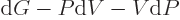
There are a number of differential expressions that are very useful
in doing thermodynamics. The primary one is obtained by combining the
differential first law (11.11) with the differential second
law (11.19) for reversible processes:
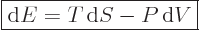 |
(11.23) |
This no longer involves the heat transferred from the surroundings,
just state variables of the system itself. The equivalent one using the
enthalpy instead of the internal energy  is
is
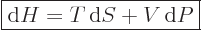 |
(11.24) |
The differentials of the Helmholtz and Gibbs free energies are, after cleaning
up with the two expressions immediately above:
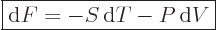 |
(11.25) |
and
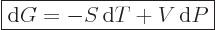 |
(11.26) |
Expression (11.25) shows that the work obtainable in an
isothermal reversible process is given by the decrease in Helmholtz
free energy. That is why Helmholtz called it “free
energy” in the first place. The Gibbs free energy is
applicable to steady flow devices such as compressors and turbines;
the first law for these devices must be corrected for the “flow
work” done by the pressure forces on the substance entering and
leaving the device. The effect is to turn  into
into 
 as the differential for the actual work obtainable from the device.
(This assumes that the kinetic and/or potential energy that the
substance picks up while going through the device is a not a factor.)
as the differential for the actual work obtainable from the device.
(This assumes that the kinetic and/or potential energy that the
substance picks up while going through the device is a not a factor.)
Maxwell noted that, according to the total differential of calculus,
the coefficients of the differentials in the right hand sides of
(11.23) through (11.26) must be the partial
derivatives of the quantity in the left hand side:
| |  |
|
| |
(11.27) |
| |  |
|
| |
(11.28) |
| |  |
|
| |
(11.29) |
| |  |
|
| |
(11.30) |
The final equation in each line can be verified by substituting in the
previous two and noting that the order of differentiation does not
make a difference. Those are called the “Maxwell relations.” They have a lot of practical uses. For
example, either of the final equations in the last two lines allows
the entropy to be found if the relationship between the
normal
variables  ,
,  , and
, and  is
known, assuming that at least one data point at every temperature is
already available. Even more important from an applied point of view,
the Maxwell relations allow whatever data you find about a substance
in literature to be stretched thin. Approximate the derivatives above
with difference quotients, and you can compute a host of information
not initially in your table or graph.
is
known, assuming that at least one data point at every temperature is
already available. Even more important from an applied point of view,
the Maxwell relations allow whatever data you find about a substance
in literature to be stretched thin. Approximate the derivatives above
with difference quotients, and you can compute a host of information
not initially in your table or graph.
There are two even more remarkable relations along these lines. They
follow from dividing (11.23) and (11.24) by
and rearranging so that becomes the quantity differentiated. That
produces
![\begin{displaymath}
\begin{array}[b]{r}
\displaystyle
\left(\frac{\partial S}...
... \left(\frac{\partial P/T}{\partial T}\right)_V
\end{array} %
\end{displaymath}](img2461.gif) |
(11.31) |
![\begin{displaymath}
\begin{array}[b]{r}
\displaystyle
\left(\frac{\partial S}...
... \left(\frac{\partial V/T}{\partial T}\right)_P
\end{array} %
\end{displaymath}](img2462.gif) |
(11.32) |
What is so remarkable is the final equation in each case: they do not
involve entropy in any way, just the normal
variables
, , , , and . Merely
because entropy exists, there must be relationships between
these variables which seemingly have absolutely nothing to do with the
second law.
As an example, consider an ideal gas, more precisely, any substance
that satisfies the ideal gas law
 |
(11.33) |
The constant  is called the specific gas constant; it can be
computed from the ratio of the Boltzmann constant
is called the specific gas constant; it can be
computed from the ratio of the Boltzmann constant  and the mass
of a single molecule
and the mass
of a single molecule  . Alternatively, it can be computed from the
“universal gas constant”
. Alternatively, it can be computed from the
“universal gas constant” 
 and the
molar mass
and the
molar mass 
 . For an ideal gas like that, the
equations above show that the internal energy and enthalpy are
functions of temperature only. And then so are the specific heats
. For an ideal gas like that, the
equations above show that the internal energy and enthalpy are
functions of temperature only. And then so are the specific heats
 and
and  , because those are their temperature derivatives:
 |
(11.34) |
(The final relation is because 


 with
with  and
and 
 .) Ideal gas tables can therefore be tabulated by
temperature only, there is no need to include a second independent
variable. You might think that entropy should be tabulated against
both varying temperature and varying pressure, because it does depend
on both pressure and temperature. However, the Maxwell equation
(11.30) may be used to find the entropy at any pressure as
long as it is listed for just one pressure, say for one bar.
.) Ideal gas tables can therefore be tabulated by
temperature only, there is no need to include a second independent
variable. You might think that entropy should be tabulated against
both varying temperature and varying pressure, because it does depend
on both pressure and temperature. However, the Maxwell equation
(11.30) may be used to find the entropy at any pressure as
long as it is listed for just one pressure, say for one bar.
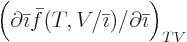
There is a sleeper among the Maxwell equations; the very first one, in
(11.27). Turned on its head, it says that
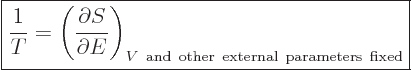 |
(11.35) |
This can be used as a definition of temperature. Note that in
taking the derivative, the volume of the box, the number of particles,
and other external parameters, like maybe an external magnetic field,
must be held constant. To understand qualitatively why the above
derivative defines a temperature, consider two systems  and
and  for
which has the larger temperature according to the definition
above. If these two systems are brought into thermal contact, then
net messiness increases when energy flows from high temperature system
to low temperature system , because system ,
with the higher value of the derivative, increases its entropy more
than decreases its.
for
which has the larger temperature according to the definition
above. If these two systems are brought into thermal contact, then
net messiness increases when energy flows from high temperature system
to low temperature system , because system ,
with the higher value of the derivative, increases its entropy more
than decreases its.
Of course, this new definition of temperature is completely consistent
with the ideal gas one; it was derived from it. However, the new
definition also works fine for negative temperatures. Assume a system
has a negative temperature according to he definition above. Then
its messiness (entropy) increases if it gives up heat. That is in stark contrast to normal substances
at positive temperatures that increase in messiness if they take in heat. So assume that system is brought into thermal
contact with a normal system at a positive temperature. Then
will give off heat to , and both systems increase their
messiness, so everyone is happy. It follows that will give off
heat however hot is the normal system it is brought into contact with.
While the temperature of may be negative, it is hotter than any
substance with a normal positive temperature!
And now the big question: what is that “chemical potential” you hear so much about? Nothing new,
really. For a pure substance with a single constituent like this
chapter is supposed to discuss, the chemical potential is just the
specific Gibbs free energy on a molar basis, 
 . More generally, if there is more than one
constituent the chemical potential
. More generally, if there is more than one
constituent the chemical potential  of each constituent
  is best defined as
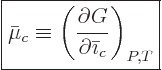 |
(11.36) |
(If there is only one constituent, then 
 and the derivative does indeed produce . Note that an
intensive quantity like , when considered to be a
function of , , and
and the derivative does indeed produce . Note that an
intensive quantity like , when considered to be a
function of , , and  , only depends
on the two intensive variables and , not on the amount of
particles present.) If there is more than one
constituent, and assuming that their Gibbs free energies simply add
up, as in
, only depends
on the two intensive variables and , not on the amount of
particles present.) If there is more than one
constituent, and assuming that their Gibbs free energies simply add
up, as in
then the chemical potential of each constituent is simply
the molar specific Gibbs free energy  of that constituent,
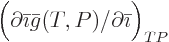
The partial derivatives described by the chemical potentials are
important for figuring out the stable equilibrium state a system
will achieve in an isothermal, isobaric, environment, i.e. in an
environment that is at constant temperature and pressure. As noted
earlier in this section, the Gibbs free energy must be as small as it
can be in equilibrium at a given temperature and pressure. Now
according to calculus, the full differential for a change in Gibbs
free energy is
The first two partial derivatives, which keep the number of particles
fixed, were identified in the discussion of the Maxwell equations as
and ; also the partial derivatives with respect to
the numbers of particles of the constituent have been defined as the
chemical potentials . Therefore more shortly,
 |
(11.37) |
This generalizes (11.26) to the case that the numbers of
constituents change. At equilibrium at given temperature and
pressure, the Gibbs energy must be minimal. It means that  must be zero whenever
  0, regardless of any
infinitesimal changes in the amounts of the constituents. That gives
a condition on the fractions of the constituents present.
0, regardless of any
infinitesimal changes in the amounts of the constituents. That gives
a condition on the fractions of the constituents present.
Note that there are typically constraints on the changes
 in the amounts of the constituents. For example, in
a liquid-vapor “phase equilibrium,” any additional amount of particles
in the amounts of the constituents. For example, in
a liquid-vapor “phase equilibrium,” any additional amount of particles
 that condenses to liquid must equal the
amount
that condenses to liquid must equal the
amount  of particles that disappears from the
vapor phase. (The subscripts follow the unfortunate convention
liquid=fluid=f and vapor=gas=g. Don’t ask.) Putting this
relation in (11.37) it can be seen that the liquid and vapor
phase must have the same chemical potential,
of particles that disappears from the
vapor phase. (The subscripts follow the unfortunate convention
liquid=fluid=f and vapor=gas=g. Don’t ask.) Putting this
relation in (11.37) it can be seen that the liquid and vapor
phase must have the same chemical potential, 
 . Otherwise the Gibbs free energy would get
smaller when more particles enter whatever is the phase of lowest
chemical potential and the system would collapse completely into that
phase alone.
. Otherwise the Gibbs free energy would get
smaller when more particles enter whatever is the phase of lowest
chemical potential and the system would collapse completely into that
phase alone.
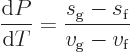
The equality of chemical potentials suffices to derive the famous
Clausius-Clapeyron equation relating pressure changes under two-phase,
or “saturated,” conditions to the corresponding temperature
changes. For, the changes in chemical potentials must be equal too,

 , and substituting in
the differential (11.26) for the Gibbs free energy, taking
it on a molar basis since ,
, and substituting in
the differential (11.26) for the Gibbs free energy, taking
it on a molar basis since ,
and rearranging gives the Clausius-Clapeyron equation:
Note that since the right-hand side is a ratio, it does not make a
difference whether you take the entropies and volumes on a molar basis
or on a mass basis. The mass basis is shown since that is how you
will typically find the entropy and volume tabulated. Typical
engineering thermodynamic textbooks will also tabulate 
 and
and 
 , making the formula above very
convenient.
, making the formula above very
convenient.
In case your tables do not have the entropies of the liquid and vapor
phases, they often still have the “latent heat of vaporization,” also known as “enthalpy of vaporization” or similar, and in engineering
thermodynamics books typically indicated by  . That
is the difference between the enthalpy of the saturated liquid and
vapor phases,
. That
is the difference between the enthalpy of the saturated liquid and
vapor phases,  . If
saturated liquid is turned into saturated vapor by adding heat under
conditions of constant pressure and temperature, (11.24)
shows that the change in enthalpy equals
. If
saturated liquid is turned into saturated vapor by adding heat under
conditions of constant pressure and temperature, (11.24)
shows that the change in enthalpy equals
 . So the Clausius-Clapeyron equation
can be rewritten as
. So the Clausius-Clapeyron equation
can be rewritten as
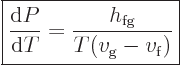 |
(11.38) |
Because  is the heat added, the physical meaning of the latent
heat of vaporization is the heat needed to turn saturated liquid into
saturated vapor while keeping the temperature and pressure constant.
is the heat added, the physical meaning of the latent
heat of vaporization is the heat needed to turn saturated liquid into
saturated vapor while keeping the temperature and pressure constant.
For chemical reactions, like maybe
the changes in the amounts of the constituents are related as
where  is the additional number of times the forward
reaction takes place from the starting state. The constants 2,
1, and 2 are called the “stoichiometric coefficients.” They can be used when applying
the condition that at equilibrium, the change in Gibbs energy due to
an infinitesimal amount of further reactions must be
zero.
is the additional number of times the forward
reaction takes place from the starting state. The constants 2,
1, and 2 are called the “stoichiometric coefficients.” They can be used when applying
the condition that at equilibrium, the change in Gibbs energy due to
an infinitesimal amount of further reactions must be
zero.
However, chemical reactions are often posed in a context of constant
volume rather than constant pressure, for one because it simplifies
the reaction kinematics. For constant volume, the Helmholtz free
energy must be used instead of the Gibbs one. Does that mean that a
second set of chemical potentials is needed to deal with those
problems? Fortunately, the answer is no, the same chemical potentials
will do for Helmholtz problems. To see why, note that by definition

 , so
, so 
 , and substituting for from
(11.37), that gives
, and substituting for from
(11.37), that gives
 |
(11.39) |
Under isothermal and constant volume conditions, the first two terms
in the right hand side will be zero and will be minimal when the
differentials with respect to the amounts of particles add up to zero.
Does this mean that the chemical potentials are also specific
Helmholtz free energies, just like they are specific Gibbs free
energies? Of course the answer is no, and the reason is that the
partial derivatives of represented by the chemical potentials keep
extensive volume , instead of intensive molar specific volume
 constant. A single-constituent molar specific Helmholtz
energy
constant. A single-constituent molar specific Helmholtz
energy  can be considered to be a function
 of temperature and molar specific volume, two
intensive variables, and then
of temperature and molar specific volume, two
intensive variables, and then
 , but
, but
 does not simply produce , even if
 produces .